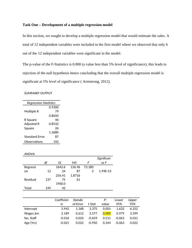
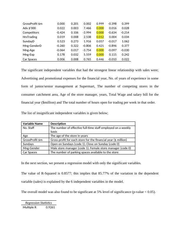
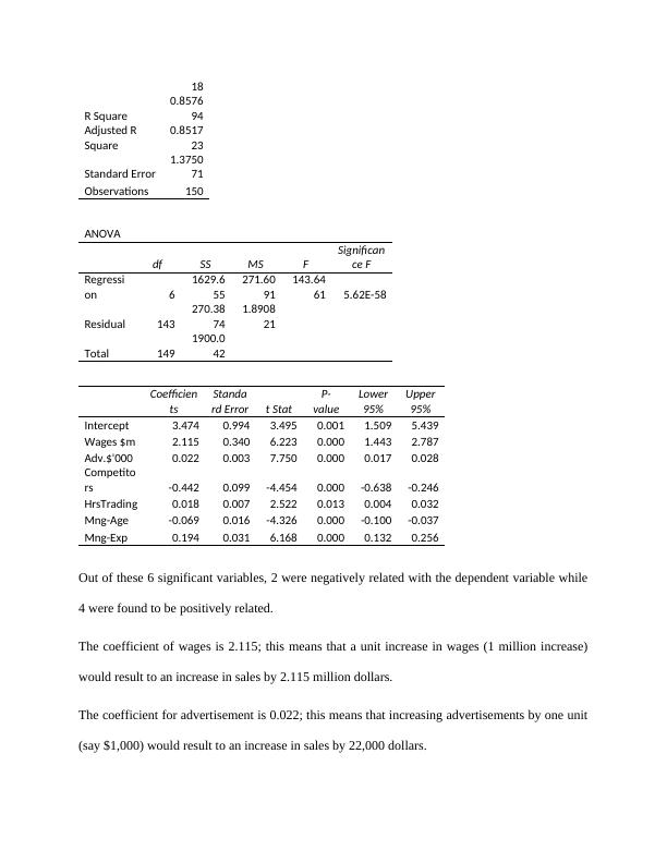
Development of a Multiple Regression Model for Sales Estimation

This article explains how to develop a multiple regression model for sales estimation using 12 independent variables. It also covers how to classify customers according to RFM and develop a sales forecast using time series analysis. The article includes regression statistics, ANOVA, coefficients, and lift ratios. It also provides a time series plot and forecast error percentage. The article is suitable for business analysis courses.

Business Analysis
Name:
Institution:
25th May 2018

Task One – Development of a multiple regression model
In this section, we sought to develop a multiple regression model that would estimate the sales. A
total of 12 independent variables were included in the first model where we observed that only 6
out of the 12 independent variables were significant in the model.
The p-value of the F-Statistics is 0.000 (a value less than 5% level of significance), this leads to
rejection of the null hypothesis hence concluding that the overall multiple regression model is
significant at 5% level of significance ( Armstrong, 2012).
SUMMARY OUTPUT
Regression Statistics
Multiple R
0.9300
79
R Square
0.8650
46
Adjusted R
Square
0.8532
26
Standard Error
1.3680
87
Observations 150
ANOVA
df SS MS F
Significan
ce F
Regressi
on 12
1643.6
24
136.96
87
73.180
3 1.99E-53
Residual 137
256.41
75
1.8716
61
Total 149
1900.0
42
Coefficien
ts
Standa
rd Error t Stat
P-
value
Lower
95%
Upper
95%
Intercept 3.942 1.168 3.375 0.001 1.632 6.252
Wages $m 2.189 0.612 3.577 0.000 0.979 3.399
No. Staff -0.016 0.024 -0.659 0.511 -0.063 0.031
Age (Yrs) -0.021 0.022 -0.950 0.344 -0.063 0.022

GrossProfit $m 0.000 0.201 0.002 0.999 -0.398 0.399
Adv.$'000 0.022 0.003 7.466 0.000 0.016 0.028
Competitors -0.424 0.106 -3.994 0.000 -0.634 -0.214
HrsTrading 0.019 0.008 2.538 0.012 0.004 0.034
SundayD 0.523 0.273 1.916 0.057 -0.017 1.062
Mng-GenderD -0.260 0.322 -0.806 0.421 -0.896 0.377
Mng-Age -0.064 0.017 -3.754 0.000 -0.097 -0.030
Mng-Exp 0.178 0.032 5.559 0.000 0.115 0.242
Car Spaces 0.006 0.008 0.765 0.446 -0.010 0.022
The significant independent variables that had the strongest linear relationship with sales were;
Advertising and promotional expenses for the financial year, No. of years of experience in some
form of junior/senior management at Supermart, The number of competing stores in the
consumer catchment area, Age of the store manager, years, Total Wage and salary bill for the
financial year ($million) and The total number of hours open for trading per week in that order.
The list of insignificant independent variables is given below;
Variable Name Description
No. Staff The number of effective full-time staff employed on a weekly
basis
Age The age of the store in years
GrossProfit $m Gross profit for each store for the financial year ($ million)
Sundays Open on Sundays (code 1); Close on Sunday (code 0)
Mng-Gender Male store manager (code 1); Female store manager (code 0)
Car Spaces The number of parking spaces available to the store
In the next section, we present a regression model with only the significant variables.
The value of R-Squared is 0.8577; this implies that 85.77% of the variation in the dependent
variable (sales) is explained by the 6 independent variables in the model.
The overall model was also found to be significant at 5% level of significance (p-value < 0.05).
Regression Statistics
Multiple R 0.9261

18
R Square
0.8576
94
Adjusted R
Square
0.8517
23
Standard Error
1.3750
71
Observations 150
ANOVA
df SS MS F
Significan
ce F
Regressi
on 6
1629.6
55
271.60
91
143.64
61 5.62E-58
Residual 143
270.38
74
1.8908
21
Total 149
1900.0
42
Coefficien
ts
Standa
rd Error t Stat
P-
value
Lower
95%
Upper
95%
Intercept 3.474 0.994 3.495 0.001 1.509 5.439
Wages $m 2.115 0.340 6.223 0.000 1.443 2.787
Adv.$'000 0.022 0.003 7.750 0.000 0.017 0.028
Competito
rs -0.442 0.099 -4.454 0.000 -0.638 -0.246
HrsTrading 0.018 0.007 2.522 0.013 0.004 0.032
Mng-Age -0.069 0.016 -4.326 0.000 -0.100 -0.037
Mng-Exp 0.194 0.031 6.168 0.000 0.132 0.256
Out of these 6 significant variables, 2 were negatively related with the dependent variable while
4 were found to be positively related.
The coefficient of wages is 2.115; this means that a unit increase in wages (1 million increase)
would result to an increase in sales by 2.115 million dollars.
The coefficient for advertisement is 0.022; this means that increasing advertisements by one unit
(say $1,000) would result to an increase in sales by 22,000 dollars.

The coefficient for competition is -0.442; this means that a unit increase in the number of
competitors would result to a decrease in sales by 442,000 dollars.
The coefficient of trading hours is 0.018; this means that a unit increase in trading hours would
result to an increase in sales by 18,000 dollars.
The coefficient for age of the store manager -0.069; this means that a unit increase in the age of
the store manager would result to a decrease in sales by 69,000 dollars.
Lastly, the coefficient of mng-exp is 0.194; this means that a unit increase in the experience of
the management would result to an increase in sales by 194,000 dollars.
The final regression equation model would therefore be like the one shown below;
Sales=3.474+ 2.115 ( wages ) +0.022 ( advertisemnets ) −0.442 ( comeptitors ) +0.018 ( trading hrs ) −0.069 ( mng age ) +
Testing multicollinearity
We tested whether there any potential multi-collinearity problems. To do this we had to compute
the tolerance and VIF.
Tolerance=1−R2 → 1−0.8577=0.1423
VIF= 1
Tolerance → 1
0.1423 =7.0274
Since the VIF is greater than 4 then there could be potential of multi-collinearity problems
(O’Brien, 2007). The independent variables with collinearity problems are advertisements and
wages; competitors and hours of trading.
Estimation

What would be the sales for a five year old store with 50 staff and 50 car spaces that is open for
100 hours per week including Sunday, managed by a 35 year old female manager with five years
of experience, that pays $2.5 million on wages, spends $150,000 on advertising, reports $1
million gross profit, with two competitor stores? [Note, only use the values that you have found
to be significant (α set at 0.05) contributors to the behavior of the dependent measure].
Sales=3.474+ 2.115 ( wages ) +0.022 ( advertisemnets ) −0.442 ( comeptitors ) +0.018 ( trading hrs ) −0.069 ( mng age ) +
wages=2.5, advertisemnets=150, comeptitors=2, trading hrs=100, mng age=35, mng exp ¿ 5
Substituting the values into the regression equation model yields;
Sales=3.474+2.115 ( 2.5 )+0.022 ( 150 ) −0.442 ( 2 )+ 0.018 ( 100 )−0.069 ( 35 ) +0.194 ( 5 ) =11.5325
Thus the sales given the input values is 11.5325 million dollars.
Task Two – Classifying customers according to RFM
Total net revenue of all customers without RFM coding
This is the sum of net revenues for all the customers and it is given as $57,594.22.
Net revenue generated by the top 10% of the customers under RFM
This is the sum of net revenues for the top 10% of customers under RFM (first 300 customers
when arranged from descending order of the RFM scores) and the value is given as $733.04
Net revenue generated by the top 20% of the customers under RFM
This is the sum of net revenues for the top 20% of customers under RFM (first 600 customers
when arranged from descending order of the RFM scores) and the value is given as $1830.94.

Response rate of the top 10% customers under RFM
This is the percentage of customer who responded and are in the top 10% of customers under
RFM (first 300 customers when arranged from descending order of the RFM scores)
Response rate= 58
300 ∗100=19.33 %
Response rate of the top 20% customers under RFM
This is the percentage of customer who responded and are in the top 20% of customers under
RFM (first 600 customers when arranged from descending order of the RFM scores)
Response rate=133
600∗100=22.17 %
Lift ratio for the top 10% and 20% customers under RFM
This is the ratio of target response divided by average response (Thomas, 2003).
For the top 10%
Lift ratio=300
58 =5.1724
For the top 20%
Lift ratio=600
133 =4.5112

Lift Chart
Figure 1: Lift chart for the response rate

Figure 2: Gain chart for the response rate
Task Three – Developing sales forecast
Figure 3: Time series plot for the sales
As can be seen from the plot, almost linear trend emerges, indicating that the company’s sales
enjoyed a steady growth over the years (approximately 3 times more sales have been made in
2018 than in 2015).

Forecasting error
We computed forecast error % by considering the differences in the actual sales and the forecast
sales (French, 2017).
Forecast error %=∑ |A−F |
∑ A = 2236.92
11253.6∗100 %=19.88 %
The forecast error was found to be 19.88% which is not large enough hence showing that the
model forecasts the sales almost accurately.
R2 value of the model
The value of R-Squared for the model was found to be 0.7301; this implies that 73.01% of the
variation in the dependent variable (sales) is explained by the change in time (Magee, 2000).
SUMMARY OUTPUT
Regression Statistics
Multiple R
0.8544
61
R Square
0.7301
03
Adjusted R
Square
0.7221
65
Standard
Error
78.504
9
Observations 36
ANOVA
df SS MS F
Significa
nce F
Regressi
on 1
566837
.1
566837
.1
91.973
92 3.37E-11
Residual 34
209542
.7
6163.0
2
Total 35 776379

.8
Coefficients
Standard
Error t Stat P-value
Lower
95%
Upper
95%
Intercept 89.13714 26.72317 3.335576 0.002068 34.82913 143.4452
Period 12.07907 1.259509 9.590304 3.37E-11 9.519443 14.6387
Prediction of the next time period
The regression model is given as;
^y=89.1371+12.0791 t
The next time period is t = 37 hence the forecast sales is;
^y=89.1371+12.0791 ( 37 ) =536.0638
Thus the predicted sales for the month of April 2018 is 536.0638.
References
Armstrong, J. S., 2012. Illusions in Regression Analysis. International Journal of Forecasting,
28(3), pp. 689-696.
French, J., 2017. The time traveller's CAPM. Investment Analysts Journal, 46(2), pp. 81-96.
Magee, L., 2000. R2 measures based on Wald and likelihood ratio joint significance tests. The
American Statistician, 44(5), pp. 250-253.
O’Brien, R. M., 2007. A Caution Regarding Rules of Thumb for Variance Inflation Factors.
Quality & Quantity, 41(5), pp. 673-679.

Thomas, Z., 2003. Biased graphs IV: Geometrical realizations. Journal of Combinatorial
Theory, 89(2), p. 231–297.