Assignment 1: Analysis of Multivariate Normal Distributions - STAT821
VerifiedAdded on 2023/06/07
|16
|2867
|477
Homework Assignment
AI Summary
This assignment explores multivariate normal distributions, covering various aspects such as generating random vectors using the Singular Value Decomposition (SVD) method, implementing the method in R, and analyzing the resulting data. The assignment delves into the properties of multivariate normal distributions, including linear transformations and joint distributions. It also includes practical applications, such as calculating confidence intervals and performing data transformations using the Box-Cox method. The assignment uses real-world data from the "Peruhair.dat" dataset to illustrate the concepts, and the solutions provide detailed R code and interpretations of the results. The assignment concludes with an analysis of confidence intervals, and power transformation techniques to achieve normality.

Running head: Assignment 1
Assignment 1
Name of the student
Name of the University
Author Note
Assignment 1
Name of the student
Name of the University
Author Note
Paraphrase This Document
Need a fresh take? Get an instant paraphrase of this document with our AI Paraphraser
Assignment 1
Question 1:
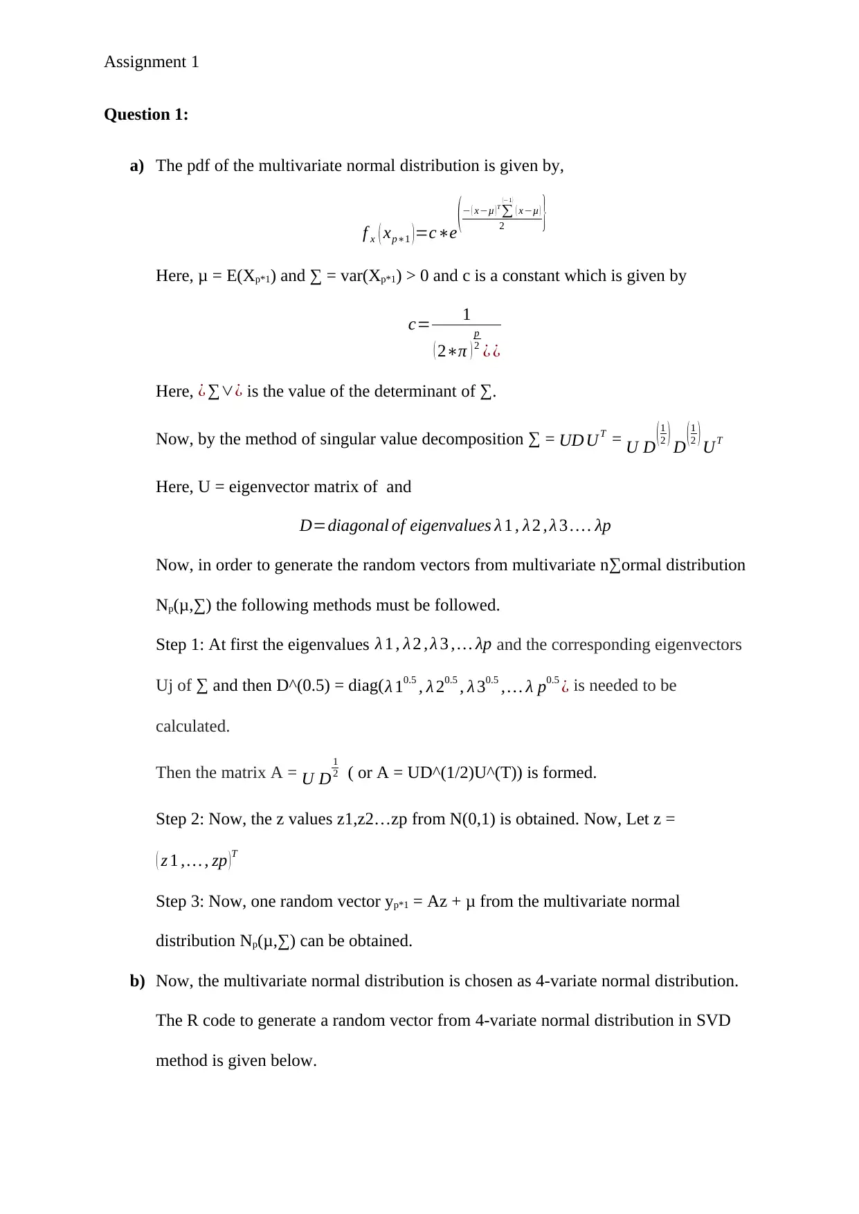
a) The pdf of the multivariate normal distribution is given by,
f x ( xp∗1 ) =c∗e
( − ( x−μ ) T
∑
(−1 )
( x−μ )
2 }
Here, μ = E(Xp*1) and ∑ = var(Xp*1) > 0 and c is a constant which is given by
c= 1
( 2∗π )
p
2 ¿ ¿
Here, ¿ ∑∨¿ is the value of the determinant of ∑.
Now, by the method of singular value decomposition ∑ = UD UT = U D (1
2 ) D (1
2 ) UT
Here, U = eigenvector matrix of and
D=diagonal of eigenvalues λ 1 , λ 2 , λ 3 … . λp
Now, in order to generate the random vectors from multivariate n∑ormal distribution
Np(μ,∑) the following methods must be followed.
Step 1: At first the eigenvalues λ 1 , λ 2 , λ 3 , … λp and the corresponding eigenvectors
Uj of ∑ and then D^(0.5) = diag( λ 10.5 , λ 20.5 , λ 30.5 , … λ p0.5 ¿ is needed to be
calculated.
Then the matrix A = U D
1
2 ( or A = UD^(1/2)U^(T)) is formed.
Step 2: Now, the z values z1,z2…zp from N(0,1) is obtained. Now, Let z =
( z 1 , … , zp )T
Step 3: Now, one random vector yp*1 = Az + μ from the multivariate normal
distribution Np(μ,∑) can be obtained.
b) Now, the multivariate normal distribution is chosen as 4-variate normal distribution.
The R code to generate a random vector from 4-variate normal distribution in SVD
method is given below.
Question 1:
a) The pdf of the multivariate normal distribution is given by,
f x ( xp∗1 ) =c∗e
( − ( x−μ ) T
∑
(−1 )
( x−μ )
2 }
Here, μ = E(Xp*1) and ∑ = var(Xp*1) > 0 and c is a constant which is given by
c= 1
( 2∗π )
p
2 ¿ ¿
Here, ¿ ∑∨¿ is the value of the determinant of ∑.
Now, by the method of singular value decomposition ∑ = UD UT = U D (1
2 ) D (1
2 ) UT
Here, U = eigenvector matrix of and
D=diagonal of eigenvalues λ 1 , λ 2 , λ 3 … . λp
Now, in order to generate the random vectors from multivariate n∑ormal distribution
Np(μ,∑) the following methods must be followed.
Step 1: At first the eigenvalues λ 1 , λ 2 , λ 3 , … λp and the corresponding eigenvectors
Uj of ∑ and then D^(0.5) = diag( λ 10.5 , λ 20.5 , λ 30.5 , … λ p0.5 ¿ is needed to be
calculated.
Then the matrix A = U D
1
2 ( or A = UD^(1/2)U^(T)) is formed.
Step 2: Now, the z values z1,z2…zp from N(0,1) is obtained. Now, Let z =
( z 1 , … , zp )T
Step 3: Now, one random vector yp*1 = Az + μ from the multivariate normal
distribution Np(μ,∑) can be obtained.
b) Now, the multivariate normal distribution is chosen as 4-variate normal distribution.
The R code to generate a random vector from 4-variate normal distribution in SVD
method is given below.
Assignment 1
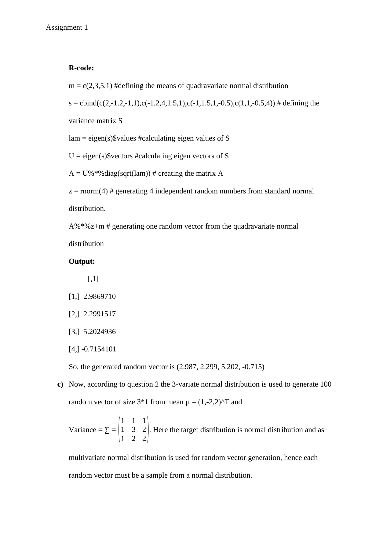
R-code:
m = c(2,3,5,1) #defining the means of quadravariate normal distribution
s = cbind(c(2,-1.2,-1,1),c(-1.2,4,1.5,1),c(-1,1.5,1,-0.5),c(1,1,-0.5,4)) # defining the
variance matrix S
lam = eigen(s)$values #calculating eigen values of S
U = eigen(s)$vectors #calculating eigen vectors of S
A = U%*%diag(sqrt(lam)) # creating the matrix A
z = rnorm(4) # generating 4 independent random numbers from standard normal
distribution.
A%*%z+m # generating one random vector from the quadravariate normal
distribution
Output:
[,1]
[1,] 2.9869710
[2,] 2.2991517
[3,] 5.2024936
[4,] -0.7154101
So, the generated random vector is (2.987, 2.299, 5.202, -0.715)
c) Now, according to question 2 the 3-variate normal distribution is used to generate 100
random vector of size 3*1 from mean μ = (1,-2,2)^T and
Variance = ∑ = ( 1 1 1
1 3 2
1 2 2 ). Here the target distribution is normal distribution and as
multivariate normal distribution is used for random vector generation, hence each
random vector must be a sample from a normal distribution.
⊘ This is a preview!⊘
Do you want full access?
Subscribe today to unlock all pages.
Trusted by 1+ million students worldwide
Assignment 1
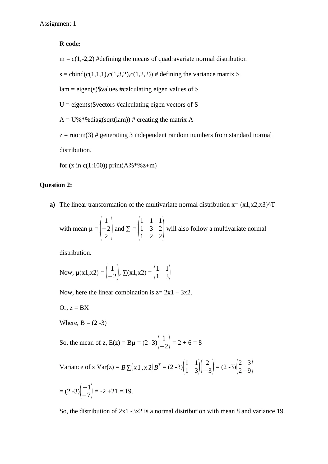
R code:
m = c(1,-2,2) #defining the means of quadravariate normal distribution
s = cbind(c(1,1,1),c(1,3,2),c(1,2,2)) # defining the variance matrix S
lam = eigen(s)$values #calculating eigen values of S
U = eigen(s)$vectors #calculating eigen vectors of S
A = U%*%diag(sqrt(lam)) # creating the matrix A
z = rnorm(3) # generating 3 independent random numbers from standard normal
distribution.
for (x in c(1:100)) print(A%*%z+m)
Question 2:
a) The linear transformation of the multivariate normal distribution x= (x1,x2,x3)^T
with mean μ = ( 1
−2
2 ) and ∑ = (1 1 1
1 3 2
1 2 2 ) will also follow a multivariate normal
distribution.
Now, μ(x1,x2) = ( 1
−2 ), ∑(x1,x2) = ( 1 1
1 3 )
Now, here the linear combination is z= 2x1 – 3x2.
Or, z = BX
Where, B = (2 -3)
So, the mean of z, E(z) = Bμ = (2 -3) ( 1
−2 ) = 2 + 6 = 8
Variance of z Var(z) = B ∑ ( x 1 , x 2 ) BT = (2 -3)( 1 1
1 3)( 2
−3 ) = (2 -3) ( 2−3
2−9 )
= (2 -3) (−1
−7 ) = -2 +21 = 19.
So, the distribution of 2x1 -3x2 is a normal distribution with mean 8 and variance 19.
Paraphrase This Document
Need a fresh take? Get an instant paraphrase of this document with our AI Paraphraser
Assignment 1
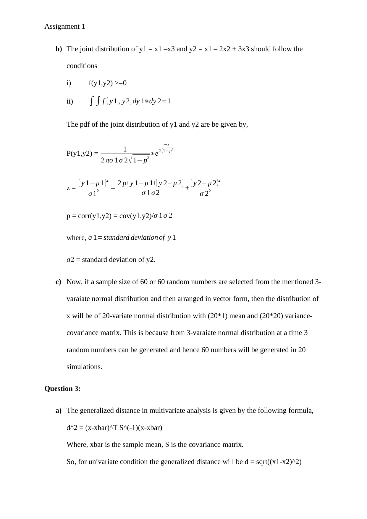
b) The joint distribution of y1 = x1 –x3 and y2 = x1 – 2x2 + 3x3 should follow the
conditions
i) f(y1,y2) >=0
ii) ∫∫ f ( y 1 , y 2 ) dy 1∗dy 2=1
The pdf of the joint distribution of y1 and y2 are be given by,
P(y1,y2) = 1
2 πσ 1 σ 2 √1− p2 ∗e
−z
2 (1− p2 )
z = ( y 1−μ 1 )2
σ 12 – 2 p ( y 1−μ 1 ) ( y 2−μ 2 )
σ 1 σ 2 + ( y 2−μ 2 )2
σ 22
p = corr(y1,y2) = cov(y1,y2)/σ 1 σ 2
where, σ 1=standard deviation of y 1
σ2 = standard deviation of y2.
c) Now, if a sample size of 60 or 60 random numbers are selected from the mentioned 3-
varaiate normal distribution and then arranged in vector form, then the distribution of
x will be of 20-variate normal distribution with (20*1) mean and (20*20) variance-
covariance matrix. This is because from 3-varaiate normal distribution at a time 3
random numbers can be generated and hence 60 numbers will be generated in 20
simulations.
Question 3:
a) The generalized distance in multivariate analysis is given by the following formula,
d^2 = (x-xbar)^T S^(-1)(x-xbar)
Where, xbar is the sample mean, S is the covariance matrix.
So, for univariate condition the generalized distance will be d = sqrt((x1-x2)^2)
Assignment 1
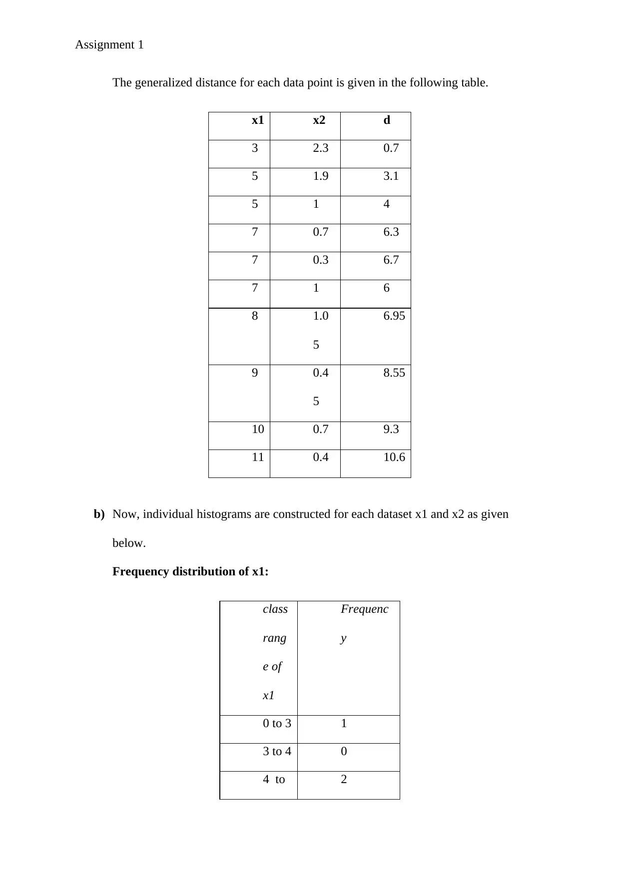
The generalized distance for each data point is given in the following table.
x1 x2 d
3 2.3 0.7
5 1.9 3.1
5 1 4
7 0.7 6.3
7 0.3 6.7
7 1 6
8 1.0
5
6.95
9 0.4
5
8.55
10 0.7 9.3
11 0.4 10.6
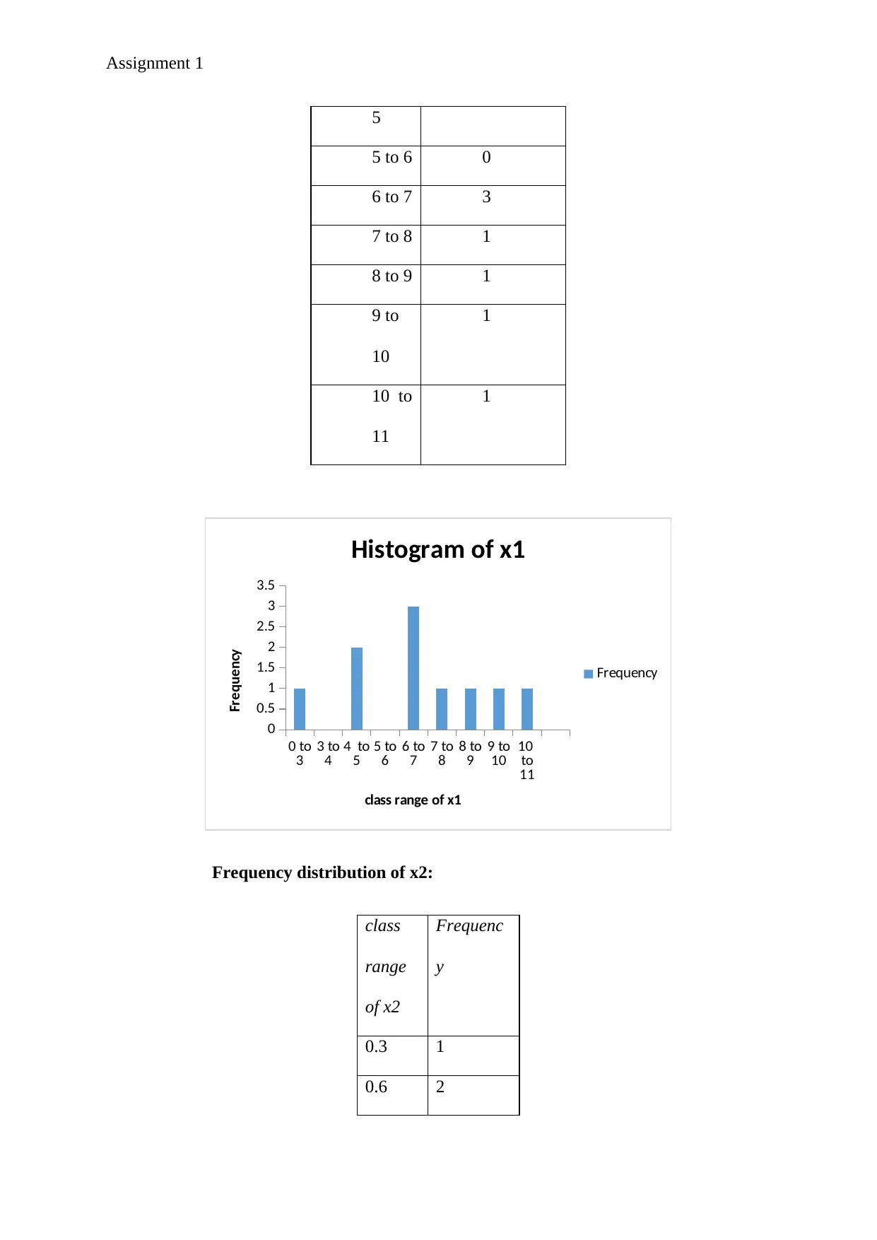
b) Now, individual histograms are constructed for each dataset x1 and x2 as given
below.
Frequency distribution of x1:
class
rang
e of
x1
Frequenc
y
0 to 3 1
3 to 4 0
4 to 2
The generalized distance for each data point is given in the following table.
x1 x2 d
3 2.3 0.7
5 1.9 3.1
5 1 4
7 0.7 6.3
7 0.3 6.7
7 1 6
8 1.0
5
6.95
9 0.4
5
8.55
10 0.7 9.3
11 0.4 10.6
b) Now, individual histograms are constructed for each dataset x1 and x2 as given
below.
Frequency distribution of x1:
class
rang
e of
x1
Frequenc
y
0 to 3 1
3 to 4 0
4 to 2
⊘ This is a preview!⊘
Do you want full access?
Subscribe today to unlock all pages.
Trusted by 1+ million students worldwide
Assignment 1
5
5 to 6 0
6 to 7 3
7 to 8 1
8 to 9 1
9 to
10
1
10 to
11
1
0 to
3 3 to
4 4 to
5 5 to
6 6 to
7 7 to
8 8 to
9 9 to
10 10
to
11
0
0.5
1
1.5
2
2.5
3
3.5
Histogram of x1
Frequency
class range of x1
Frequency
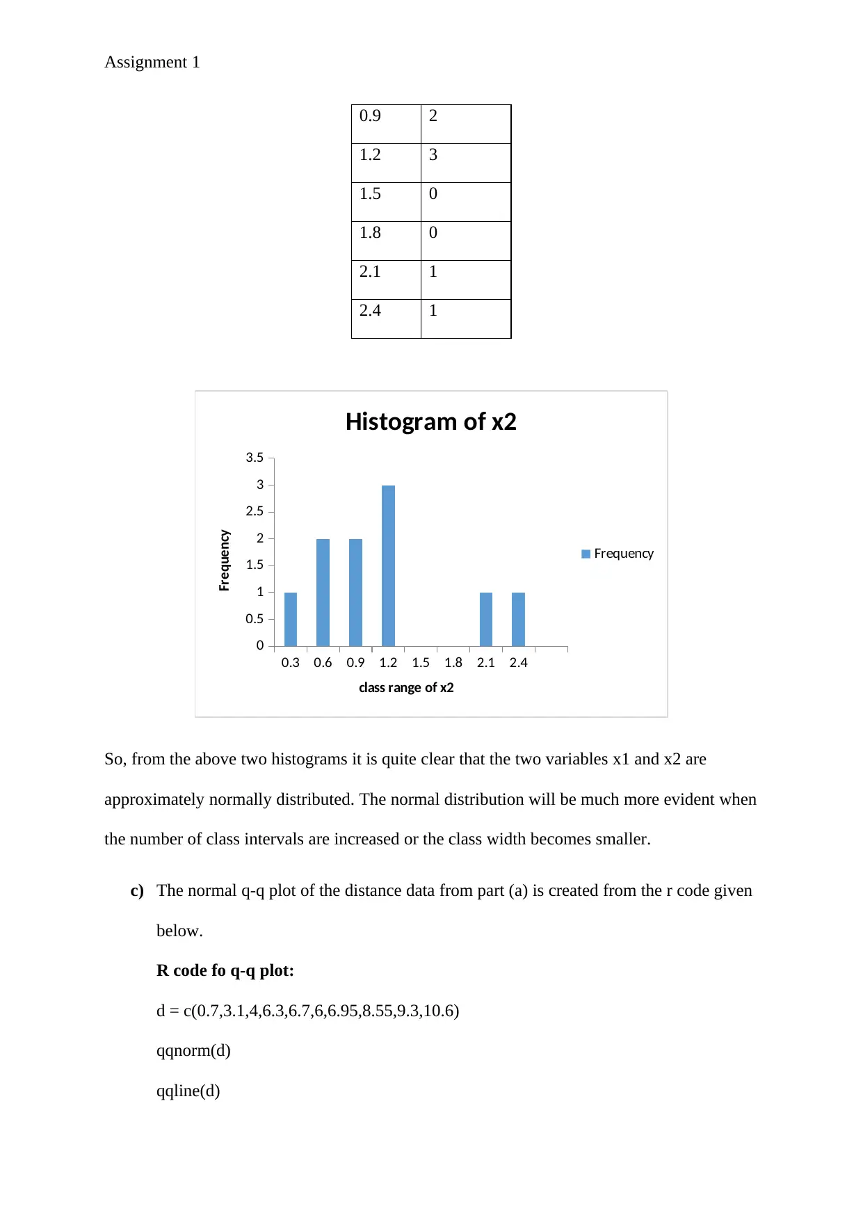
Frequency distribution of x2:
class
range
of x2
Frequenc
y
0.3 1
0.6 2
5
5 to 6 0
6 to 7 3
7 to 8 1
8 to 9 1
9 to
10
1
10 to
11
1
0 to
3 3 to
4 4 to
5 5 to
6 6 to
7 7 to
8 8 to
9 9 to
10 10
to
11
0
0.5
1
1.5
2
2.5
3
3.5
Histogram of x1
Frequency
class range of x1
Frequency
Frequency distribution of x2:
class
range
of x2
Frequenc
y
0.3 1
0.6 2
Paraphrase This Document
Need a fresh take? Get an instant paraphrase of this document with our AI Paraphraser
Assignment 1
0.9 2
1.2 3
1.5 0
1.8 0
2.1 1
2.4 1
0.3 0.6 0.9 1.2 1.5 1.8 2.1 2.4
0
0.5
1
1.5
2
2.5
3
3.5
Histogram of x2
Frequency
class range of x2
Frequency
So, from the above two histograms it is quite clear that the two variables x1 and x2 are
approximately normally distributed. The normal distribution will be much more evident when
the number of class intervals are increased or the class width becomes smaller.
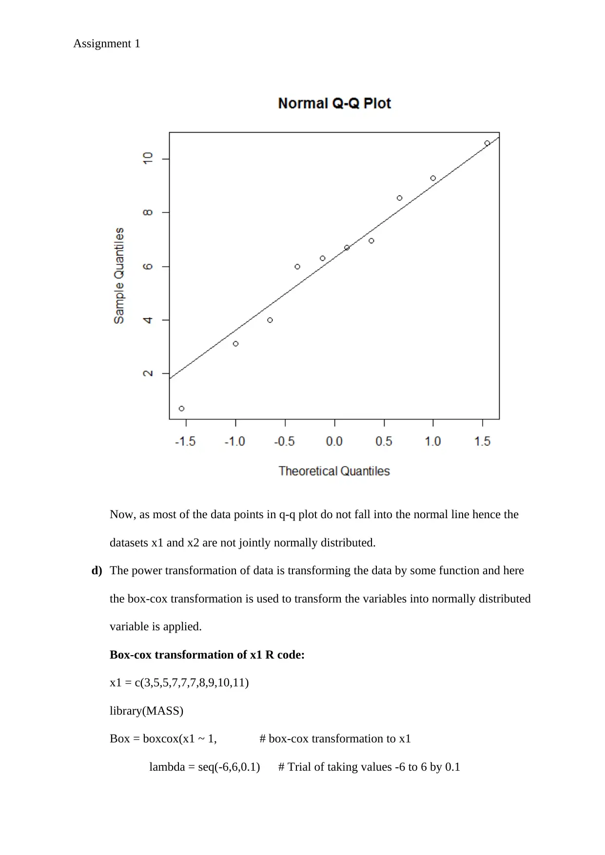
c) The normal q-q plot of the distance data from part (a) is created from the r code given
below.
R code fo q-q plot:
d = c(0.7,3.1,4,6.3,6.7,6,6.95,8.55,9.3,10.6)
qqnorm(d)
qqline(d)
0.9 2
1.2 3
1.5 0
1.8 0
2.1 1
2.4 1
0.3 0.6 0.9 1.2 1.5 1.8 2.1 2.4
0
0.5
1
1.5
2
2.5
3
3.5
Histogram of x2
Frequency
class range of x2
Frequency
So, from the above two histograms it is quite clear that the two variables x1 and x2 are
approximately normally distributed. The normal distribution will be much more evident when
the number of class intervals are increased or the class width becomes smaller.
c) The normal q-q plot of the distance data from part (a) is created from the r code given
below.
R code fo q-q plot:
d = c(0.7,3.1,4,6.3,6.7,6,6.95,8.55,9.3,10.6)
qqnorm(d)
qqline(d)
Assignment 1
Now, as most of the data points in q-q plot do not fall into the normal line hence the
datasets x1 and x2 are not jointly normally distributed.
d) The power transformation of data is transforming the data by some function and here
the box-cox transformation is used to transform the variables into normally distributed
variable is applied.
Box-cox transformation of x1 R code:
x1 = c(3,5,5,7,7,7,8,9,10,11)
library(MASS)
Box = boxcox(x1 ~ 1, # box-cox transformation to x1
lambda = seq(-6,6,0.1) # Trial of taking values -6 to 6 by 0.1
⊘ This is a preview!⊘
Do you want full access?
Subscribe today to unlock all pages.
Trusted by 1+ million students worldwide
Assignment 1
)
Cox = data.frame(Box$x, Box$y) # Create a data frame with the results
Cox2 = Cox[with(Cox, order(-Cox$Box.y)),] # Ordering the new data frame
Cox2[1,] # Display the lambda with maximum log likelihood
lambda = Cox2[1, "Box.x"] # lambda extraction
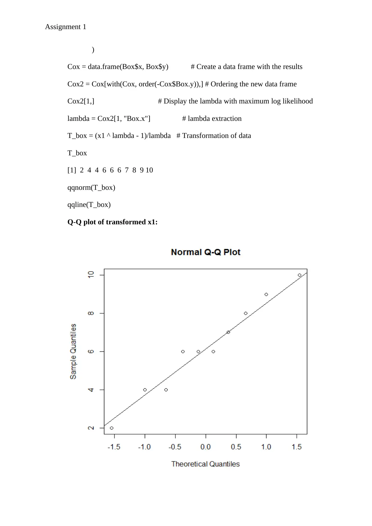
T_box = (x1 ^ lambda - 1)/lambda # Transformation of data
T_box
[1] 2 4 4 6 6 6 7 8 9 10
qqnorm(T_box)
qqline(T_box)
Q-Q plot of transformed x1:
)
Cox = data.frame(Box$x, Box$y) # Create a data frame with the results
Cox2 = Cox[with(Cox, order(-Cox$Box.y)),] # Ordering the new data frame
Cox2[1,] # Display the lambda with maximum log likelihood
lambda = Cox2[1, "Box.x"] # lambda extraction
T_box = (x1 ^ lambda - 1)/lambda # Transformation of data
T_box
[1] 2 4 4 6 6 6 7 8 9 10
qqnorm(T_box)
qqline(T_box)
Q-Q plot of transformed x1:
Paraphrase This Document
Need a fresh take? Get an instant paraphrase of this document with our AI Paraphraser
Assignment 1
Box-cox transformation of x2 R code:
x2= c(2.3,1.9,1,0.7,0.3,1,1.05,0.45,0.7,0.4)
library(MASS)
Box = boxcox(x2 ~ 1, # box-cox transformation to x2
lambda = seq(-6,6,0.1) # Trial of taking values -6 to 6 by 0.1
)
Cox = data.frame(Box$x, Box$y) # Create a data frame with the results
Cox2 = Cox[with(Cox, order(-Cox$Box.y)),] # Ordering the new data frame
Cox2[1,] # Display the lambda with maximum log likelihood
lambda = Cox2[1, "Box.x"] # lambda extraction
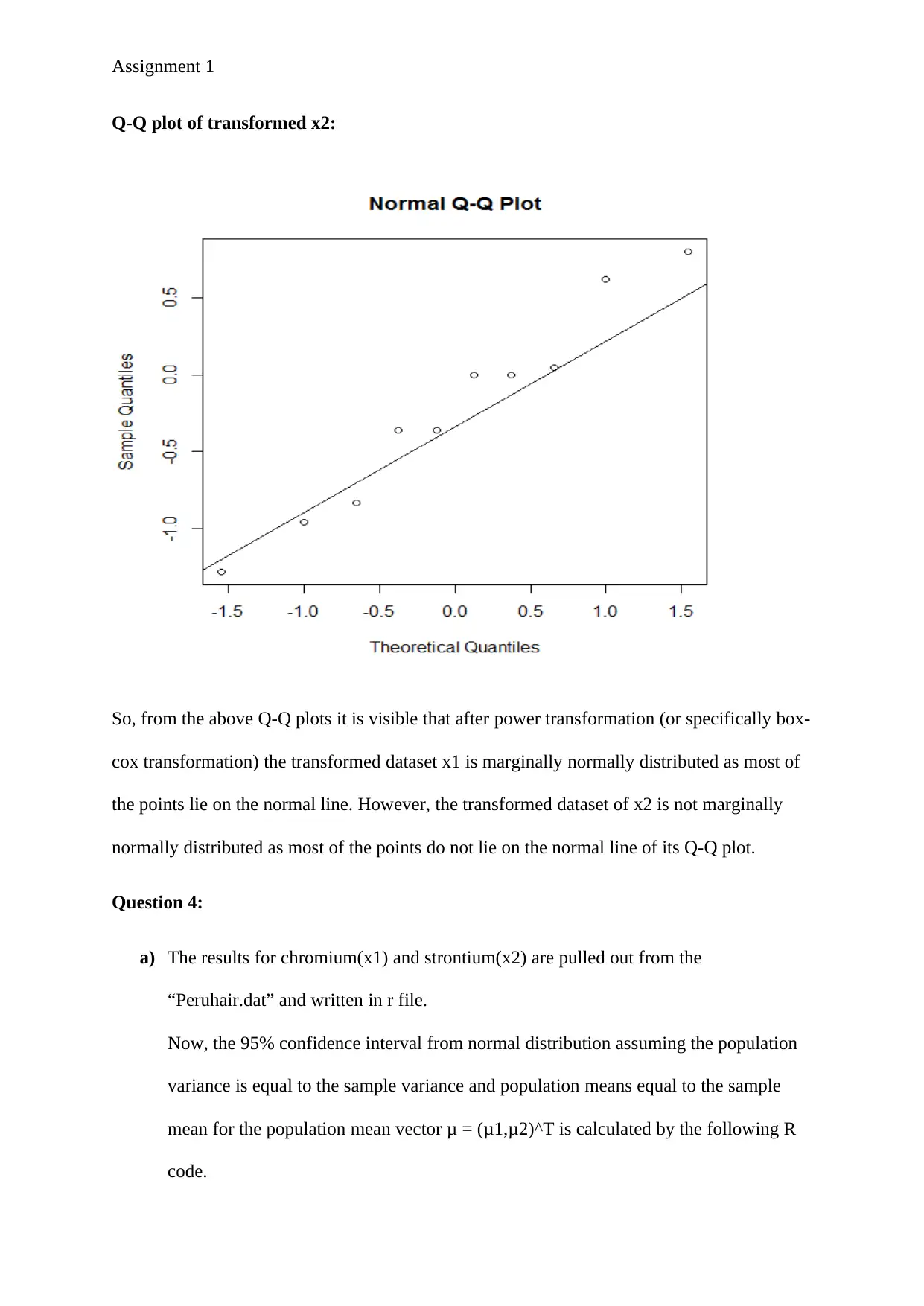
T_box = (x2 ^ lambda - 1)/lambda # Transformation of data
T_box
[1] 0.79916555 0.62168880 0.00000000 -0.36311210 -1.27944873 0.00000000
[7] 0.04867133 -0.83125420 -0.36311210 -0.95958226
qqnorm(T_box)
qqline(T_box)
Box-cox transformation of x2 R code:
x2= c(2.3,1.9,1,0.7,0.3,1,1.05,0.45,0.7,0.4)
library(MASS)
Box = boxcox(x2 ~ 1, # box-cox transformation to x2
lambda = seq(-6,6,0.1) # Trial of taking values -6 to 6 by 0.1
)
Cox = data.frame(Box$x, Box$y) # Create a data frame with the results
Cox2 = Cox[with(Cox, order(-Cox$Box.y)),] # Ordering the new data frame
Cox2[1,] # Display the lambda with maximum log likelihood
lambda = Cox2[1, "Box.x"] # lambda extraction
T_box = (x2 ^ lambda - 1)/lambda # Transformation of data
T_box
[1] 0.79916555 0.62168880 0.00000000 -0.36311210 -1.27944873 0.00000000
[7] 0.04867133 -0.83125420 -0.36311210 -0.95958226
qqnorm(T_box)
qqline(T_box)
Assignment 1
Q-Q plot of transformed x2:
So, from the above Q-Q plots it is visible that after power transformation (or specifically box-
cox transformation) the transformed dataset x1 is marginally normally distributed as most of
the points lie on the normal line. However, the transformed dataset of x2 is not marginally
normally distributed as most of the points do not lie on the normal line of its Q-Q plot.
Question 4:
a) The results for chromium(x1) and strontium(x2) are pulled out from the
“Peruhair.dat” and written in r file.
Now, the 95% confidence interval from normal distribution assuming the population
variance is equal to the sample variance and population means equal to the sample
mean for the population mean vector μ = (μ1,μ2)^T is calculated by the following R
code.
⊘ This is a preview!⊘
Do you want full access?
Subscribe today to unlock all pages.
Trusted by 1+ million students worldwide
1 out of 16
Your All-in-One AI-Powered Toolkit for Academic Success.
+13062052269
info@desklib.com
Available 24*7 on WhatsApp / Email
![[object Object]](/_next/static/media/star-bottom.7253800d.svg)
Unlock your academic potential
Copyright © 2020–2026 A2Z Services. All Rights Reserved. Developed and managed by ZUCOL.