Time Series Analysis: Forecasting Air Passenger Numbers Using ARIMA

This assignment presents a comprehensive time series analysis of the AirPassenger dataset, employing the ARIMA (Autoregressive Integrated Moving Average) model for forecasting. The analysis begins with an introduction to time series components and the rationale for using time series models...Read More

Name
Course
Date
Institution

2
Contents
• Introduction ………………………………………………………………….. 3
• Descriptive Statistics ……………………………………………………… 4
• Plots ……………………………………………….…………………………….. 5
• ARIMA Model ………………………..…………………………………….. 7
• Prediction ……………………………………………………………………… 9
• Conclusion and Recommendations ……………………………….. 10
• References …………………………………………………………………….. 11

3
Introduction
• Several statistical models are used for the prediction (forecasting) of future values
of data. The models include regression models, neural networks and time series
models. In cases where the data has a time component, the time series models
are best fit for the prediction of future values.
• Time series have three components: trend component, cyclic (seasonal)
component and the random component (Anderson, 2011).
• This research applied time series analysis on the AirPassenger dataset available in
the R Software. An ARIMA (p, d, q) model was developed and applied with
predictions made based on the resultant ARIMA model. Autocorrelation and
Partial autocorrelation graphs are used to determine the values of p and q in the
model (Zhu and Wang, 2010; Getis, 2010).

4
Descriptive Statistics
• The describe () function in the psych R package was used for the
descriptive statistics. The results of the descriptive statistics are given
in table below:
Statistic Value
Mean 280
Minimum 104
Maximum 622
Range 518
Standard Deviation 120
Kurtosis 0.57

5
Plots
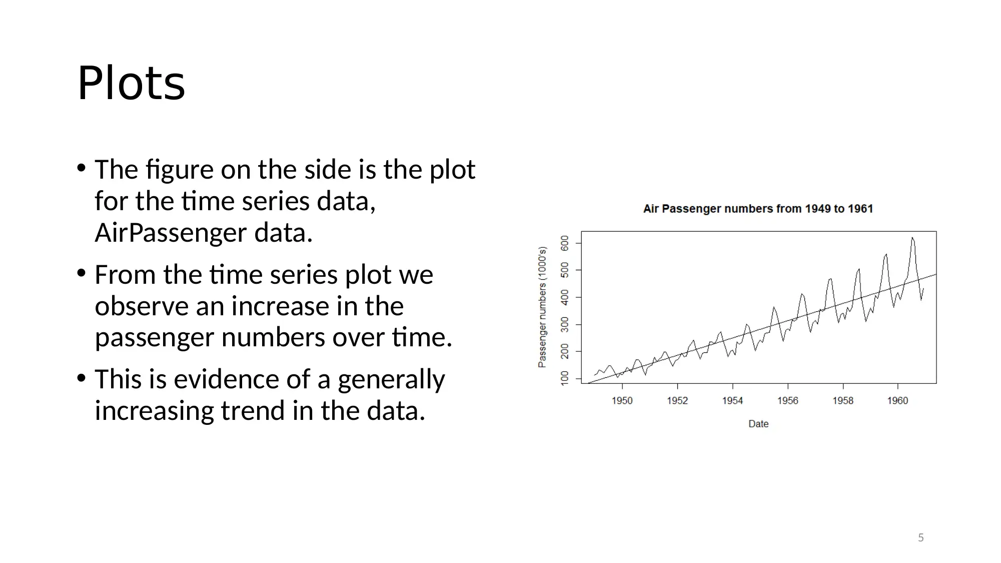
• The figure on the side is the plot
for the time series data,
AirPassenger data.
• From the time series plot we
observe an increase in the
passenger numbers over time.
• This is evidence of a generally
increasing trend in the data.

6
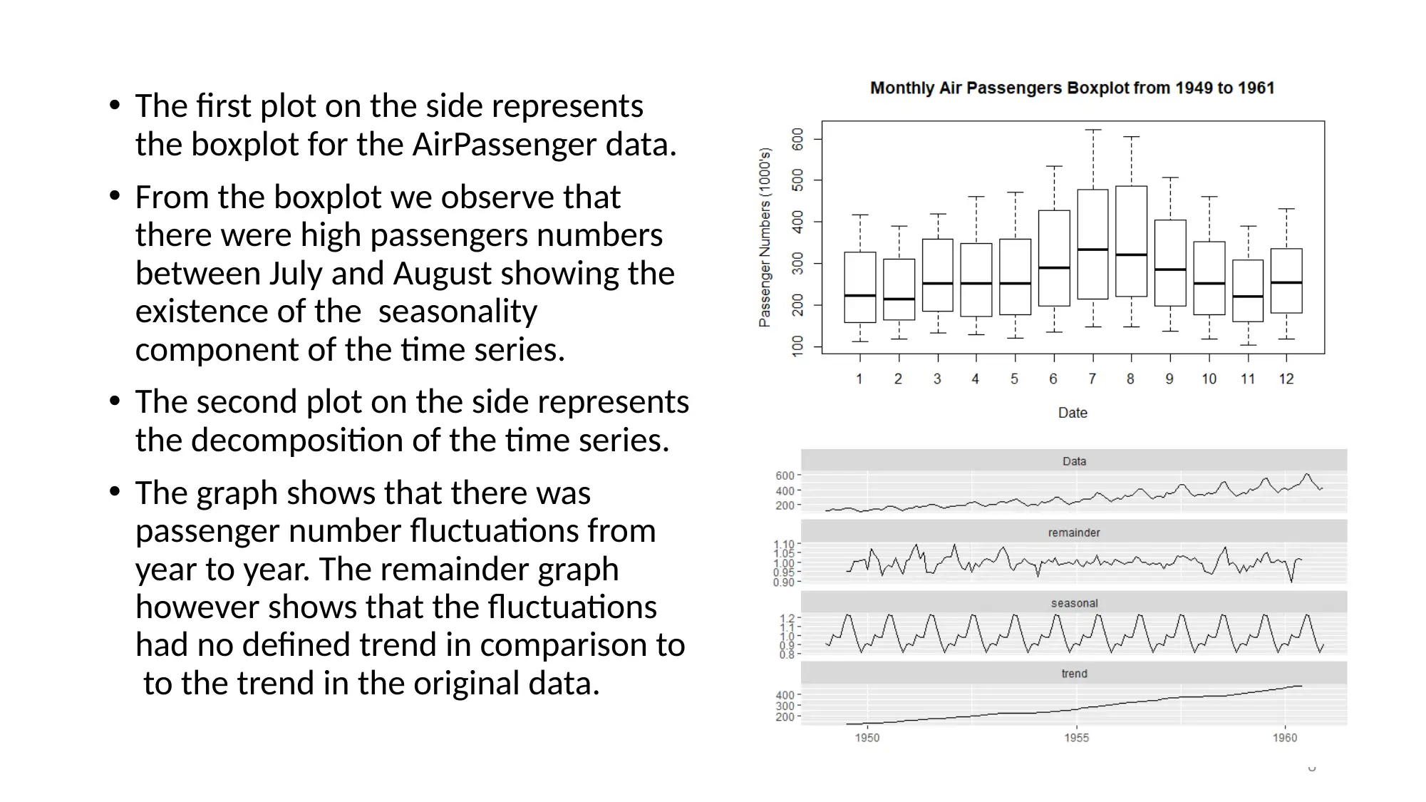
• The first plot on the side represents
the boxplot for the AirPassenger data.
• From the boxplot we observe that
there were high passengers numbers
between July and August showing the
existence of the seasonality
component of the time series.
• The second plot on the side represents
the decomposition of the time series.
• The graph shows that there was
passenger number fluctuations from
year to year. The remainder graph
however shows that the fluctuations
had no defined trend in comparison to
to the trend in the original data.

7
ARIMA Model
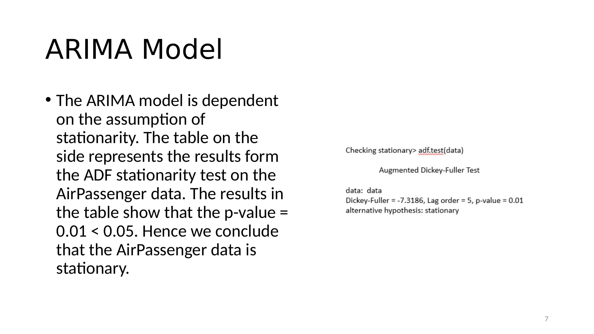
• The ARIMA model is dependent
on the assumption of
stationarity. The table on the
side represents the results form
the ADF stationarity test on the
AirPassenger data. The results in
the table show that the p-value =
0.01 < 0.05. Hence we conclude
that the AirPassenger data is
stationary.

8
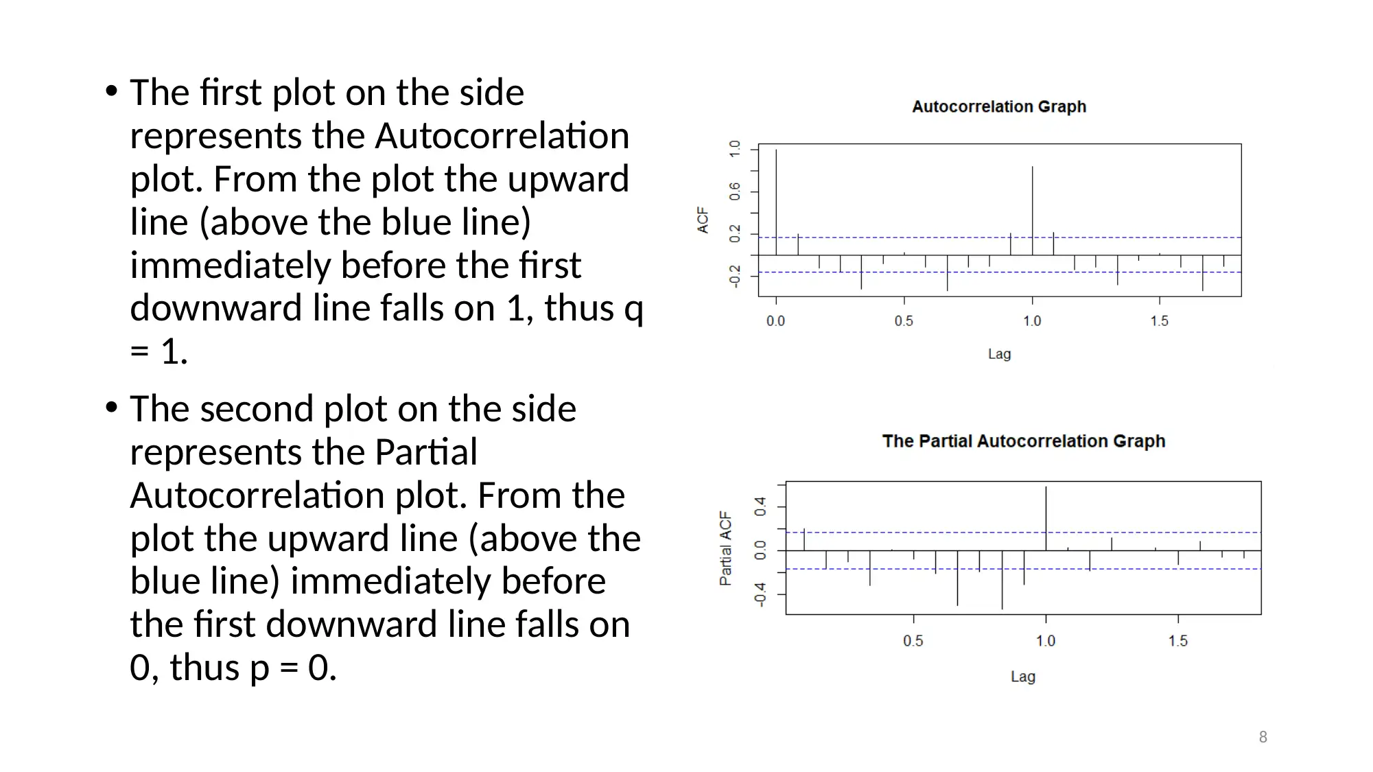
• The first plot on the side
represents the Autocorrelation
plot. From the plot the upward
line (above the blue line)
immediately before the first
downward line falls on 1, thus q
= 1.
• The second plot on the side
represents the Partial
Autocorrelation plot. From the
plot the upward line (above the
blue line) immediately before
the first downward line falls on
0, thus p = 0.

9
Prediction
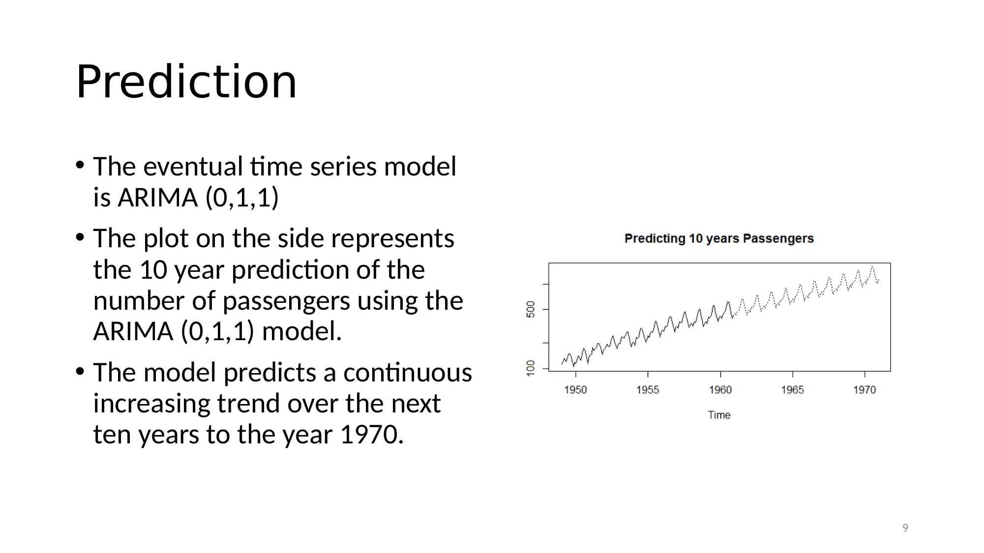
• The eventual time series model
is ARIMA (0,1,1)
• The plot on the side represents
the 10 year prediction of the
number of passengers using the
ARIMA (0,1,1) model.
• The model predicts a continuous
increasing trend over the next
ten years to the year 1970.

10
Conclusion and Recommendations
• The plot of the AirPassenger data shows a general increase in the
passenger numbers between 1949 and 1960 with peak numbers achieved
in the months of July and August.
• The ARIMA (0, 1, 1) successfully predicts the passenger numbers over the
next decade from 1960. The prediction shows a continuous increasing
trend over the 10 year period in the passenger numbers.
• Using the inferences and conclusion drawn from this research, the aviation
company can adequately prepare for increasing passenger numbers every
year over the next decade by setting up appropriate strategies. The
aviation company can also increase the flight changes in the peak months
of July and August in order to capitalize on the high passenger numbers.

11
References
Anderson, TW 2011, The statistical analysis of time series 1st edn. John Wiley & Sons,
New York.
Getis, A 2010, ‘Spatial autocorrelation’, In Handbook of applied spatial analysis (pp.
255-278), Springer, Berlin.
Marazzo, M, Scherre, R & Fernandes, E 2010, “Air transport demand and economic
growth in Brazil: A time series analysis”, Transportation Research Part E: Logistics and
Transportation Review, vol.46, no.2, pp.261-269.
Pioneer 2019, Aviation, viewed 15 September 2019 <
https://www.pioneer.com.ph/products/aviation>
Zhu, F & Wang, D 2010, “Diagnostic checking integer-valued ARCH (p) models using
conditional residual autocorrelations”, Computational Statistics & Data Analysis,
vol.54,no.2, pp.496-508.