Content of Articles Project 2022

Content of Articles

1. Shorten Grilled on Negative Gearing and Franking Credits
Labor Leader Bill Shorten has been grilled about his party's planned changes to negative
gearing and franking credits during a special episode of ABC's Q&A.
If elected on 18 May, a federal Labor government would scrap negative gearing on
investment properties from 1 January in 2020, except for newly-constructed houses.
Bill Shorten appeared on Q&A with less than two weeks to go before the May 18
election.
Bill Shorten appeared on Q&A with less than two weeks to go before the May 18
election.
ABC
Negative gearing allows property owners to claim rental losses as a tax deduction.
Speaking in front of a live studio audience in Melbourne, Mr Shorten insisted that the
changes were not tax hikes, but the removal of tax subsidies.
"You use the word tax. If I'm not giving you a subsidy for you making a loss on an
investment property, that ain't a new tax. It just means you're not getting a new subsidy,"
Mr Shorten said.
Will Labor’s negative gearing policy lead to more property owners selling then claiming
pensions? #QandA pic.twitter.com/4DH7tarWvH

— ABC Q&A (@QandA) May 6, 2019
The Opposition Leader was also confronted by a man who said he would lose 20 per cent
of his income as a result of Labor's plans to limit franking credits.
Mr Shorten said it was a "gift" paid for by millions of working Australians.
While Labor has tried to focus on health during the election campaign, its come under
pressure to explain how it will pay for its policies.
Asked to detail the cost of its climate policy, Mr Shorten dismissed it as a "dumb
question".
"You can't have a debate about climate change without talking about the cost of
inaction," he said.
"There is a cost. The bushfires, the extreme weather events, the insurance premiums."
Indigenous suicide a 'national emergency'
During the hour-long session, Mr Shorten also declared Indigenous suicide is now at the
level of a national emergency.

The Labor leader said Australia needs to redefine its relationship with its indigenous
people from one of indifference or paternalism to a true partnership.
"I think it's a national disaster, (a) national emergency," he told ABC's Q&A on Monday
night.
ELECTION19 BILL SHORTEN CAMPAIGN DAY 26
Labor Leader Bill Shorten.
AAP
"The issue of suicide is massive. But also the issue of our first Australians and the
inequality of the lives that many of them live is massive. There's an intersection."
He noted both his party and the coalition had committed to a range of suicide prevention
projects, particularly ones aimed at young people, during the lead-up to the 18 May
election.
But, he said, Labor also had a unique idea to help make sure indigenous people received
holistic solutions: making an indigenous man, Pat Dodson, the minister.
How would a Shorten government reduce Indigenous youth suicide? #QandA
pic.twitter.com/AjqpkVXpru
— ABC Q&A (@QandA) May 6, 2019

"Sometimes we judge ourselves by how many billionaires we have on the Forbes Rich
List," Mr Shorten said.
"I have a view we should judge ourselves by if we have a great disadvantage."
Mr Dodson spoke at Labor's campaign launch on Sunday, releasing the party's plans for
working with indigenous people.
These include creating a system of regional assemblies and a Voice to the national
parliament, establishing a national Makarrata commission and local truth-telling
programs, building a national resting place for the unknown warriors, and giving justice
and compensation to survivors of the stolen generation.
2. 11 Urban Myths About Franking Credits
The decision to introduce dividend imputation has provided an unforeseen benefit for
Australia, perhaps one that is still not fully appreciated by policy makers – it has made
Australian companies manage their capital more efficiently. That makes them sounder
investments.
Yet this benefit appears to be in jeopardy because the debate about the value of dividend
imputation is obscured by myths. This submission seeks to puncture these illusions in the
hope that policy makers will possess the information they need when judging the
effectiveness of a tax system that has served Australia well since 1987

Myth 1: Franking is an anachronism; Australia should modernise its tax structure
Reality: Franking’s primary benefits – avoiding double taxation, removing the incentive for
high levels of corporate debt – remain valid
Dividend imputation was introduced to avoid the unfairness of taxing company profits twice.
That motivation still stands. Without franking, the interest expense deduction would be
expected to have more influence in corporate funding. Since the introduction of franking,
Australian companies have increased their gearing levels – in line with the secular decline in
interest rates in the western world – but to a lesser extent than US companies have.
Not creating further incentives for Australian corporates to take on more debt is highly
desirable since negative gearing has created an incentive for high levels of borrowing by the
household sector:
Myth 2: Franking is all about the tax refunds
Reality: Franking’s most important influence has been on capital allocation within the
economy

Growth and innovation require that funds available for investment are channelled to the most
promising opportunities. Franking facilitates this by automatically prompting companies that
generate the most cash flow to pay it out, which allows shareholders to reinvest that cash
flow into the best opportunities. Without franking, this capital-recycling process would be
diminished due to the friction of corporate tax reducing the funds available to be reinvested.
This recycling is necessary in Australia, which is an economy of cash-flow “haves” and cash-
flow “have nots”. As the charts below show, Australia has a greater proportion of its market
comprised of larger companies. Further, smaller companies in the US tend to generate higher
returns than their counterparts in Australia. This means that Australia’s smaller companies
are more reliant on attracting the dividends flowing from the largest stocks.
Myth 3: Australia has enjoyed extended economic growth. Franking has played no part in
this
Reality: It is likely that franking has contributed to Australia’s lower economic volatility
Franking constrains corporate reinvestment. If we assume that companies will fund their best
projects first, their second-best projects second, etc., then constrained reinvestment should
result in better outcomes. If only the best projects are funded, then those projects are likely to
be more robust through the economic cycle. At the margin, this likely brings greater stability
to employment, consumer sentiment, etc.

As expected, corporate returns in Australia have improved, and have advanced more than
returns in the US:
This holds true even after excluding the anomalous mining and tech sectors:
What’s more, the quality of returns has improved, as the variance of returns has diminished
and the persistence of high returns has increased:
Myth 4: If Australian companies have higher payout ratios, it must be at the expense of
capex – but we need more investment now, not less
Reality: Relative to US companies, Australian companies pay higher dividends and also
invest more; the key difference is that Australian companies run their balance sheets more
efficiently
In this instance, it’s best to look at companies’ overall use of cash. Despite higher payouts
(and higher interest expense), Australian companies do not spend less on capex. There is no
evidence that higher payouts have led to lower levels of investment.

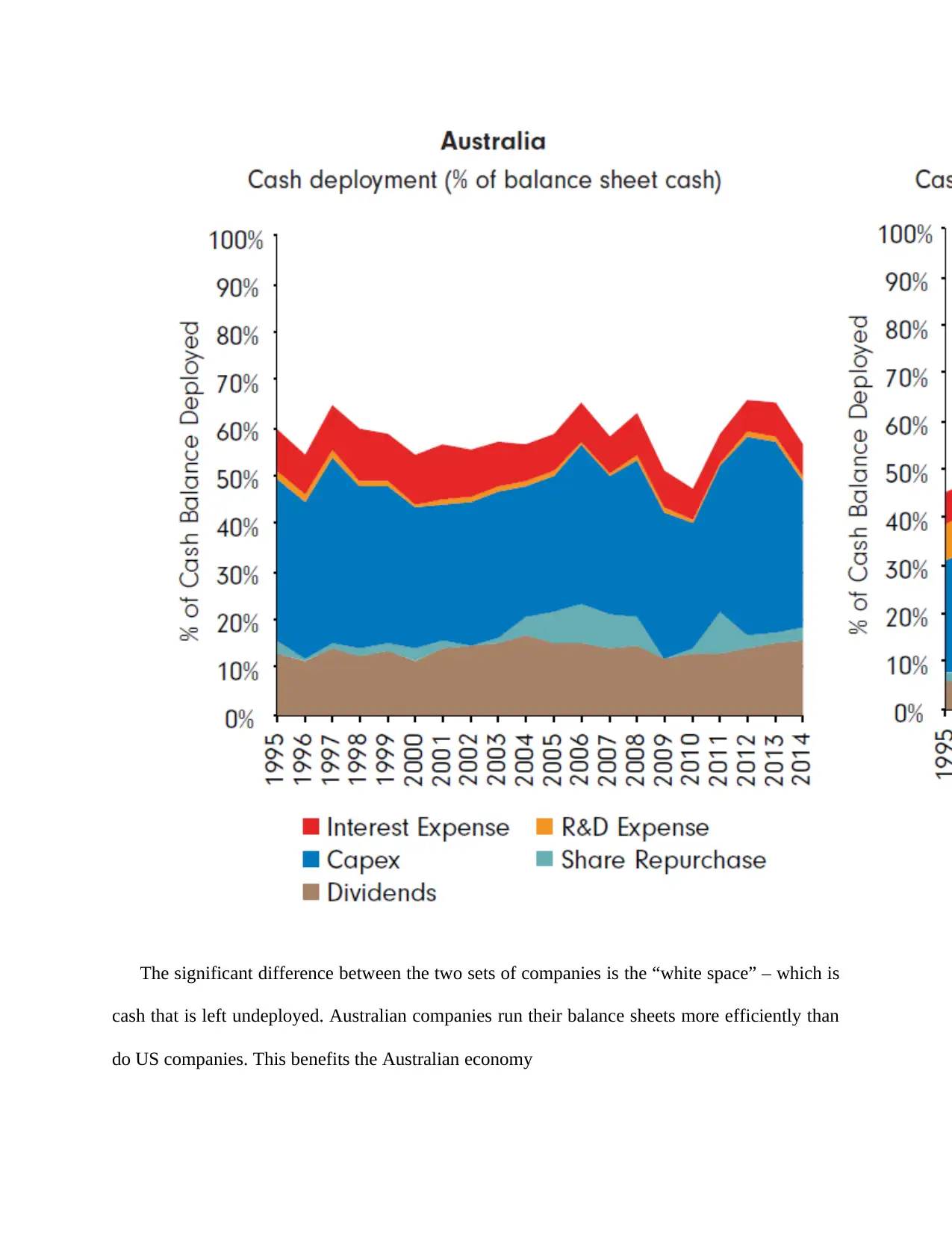
The significant difference between the two sets of companies is the “white space” – which is
cash that is left undeployed. Australian companies run their balance sheets more efficiently than
do US companies. This benefits the Australian economy

Myth 5: Franking promotes higher payouts, which reduces reinvestment and lowers
future growth
Reality: Higher payouts indicate higher future earnings growth – there is no income-
growth trade-off
Conventional wisdom holds that companies retain more earnings when growth opportunities
are ample and fruitful. Therefore, the paying out of large amounts of dividends signals a paucity
of good growth opportunities. However, academic analysis challenges this view. Arnott and
Asness (2003) used 130 years’ worth of data to show that it is high-payout firms that generate
the best earnings growth over time.
The work of Zhou and Ruland (2006) supported the Arnott and Asness conclusion. By using
data over 50 years, their paper showed that high-dividend-payout companies tend to experience
“strong, not weak, future earnings growth”.
Despite Australian companies increasing their payout ratios after the introduction of
franking, asset growth rates have increased:

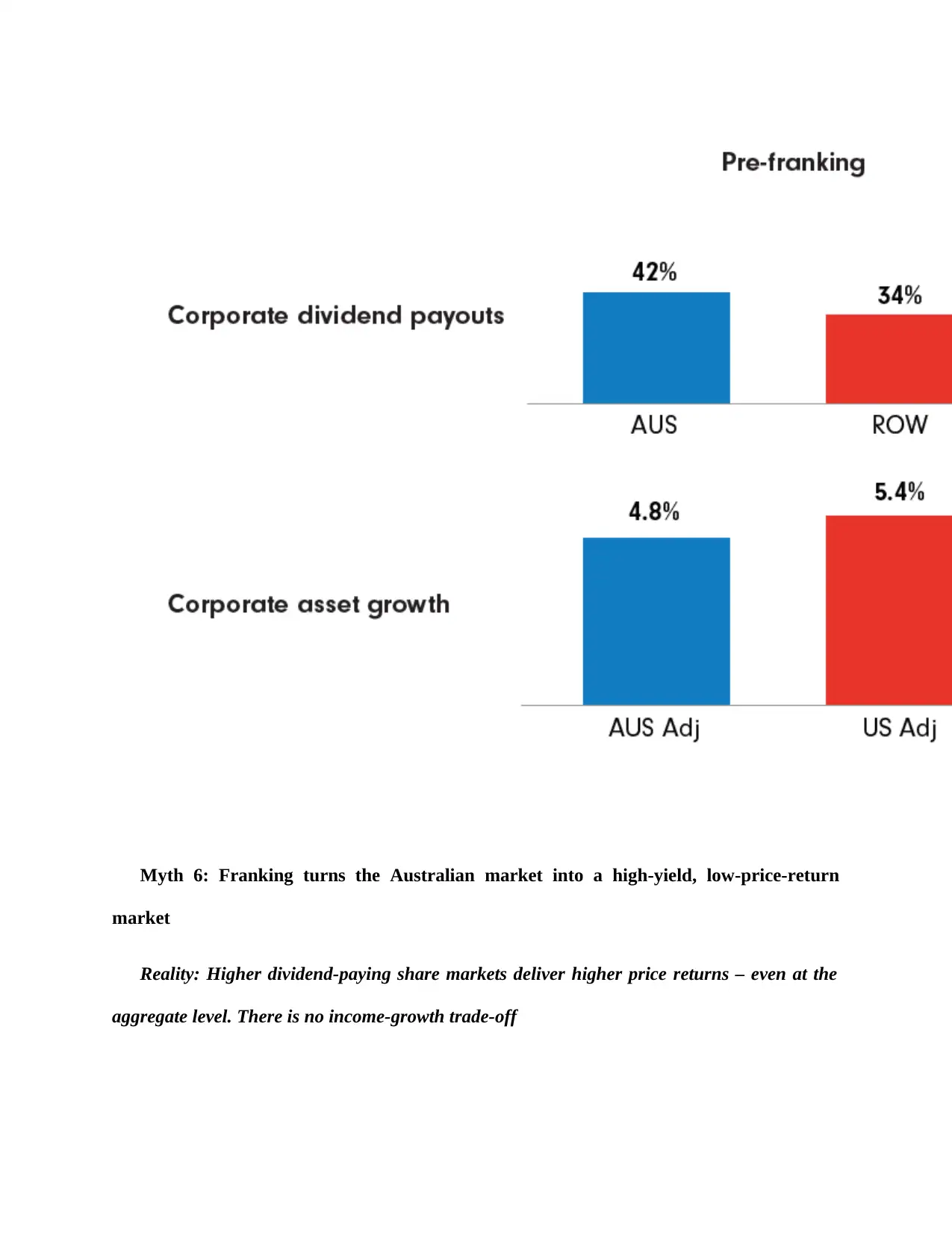
Myth 6: Franking turns the Australian market into a high-yield, low-price-return
market
Reality: Higher dividend-paying share markets deliver higher price returns – even at the
aggregate level. There is no income-growth trade-off

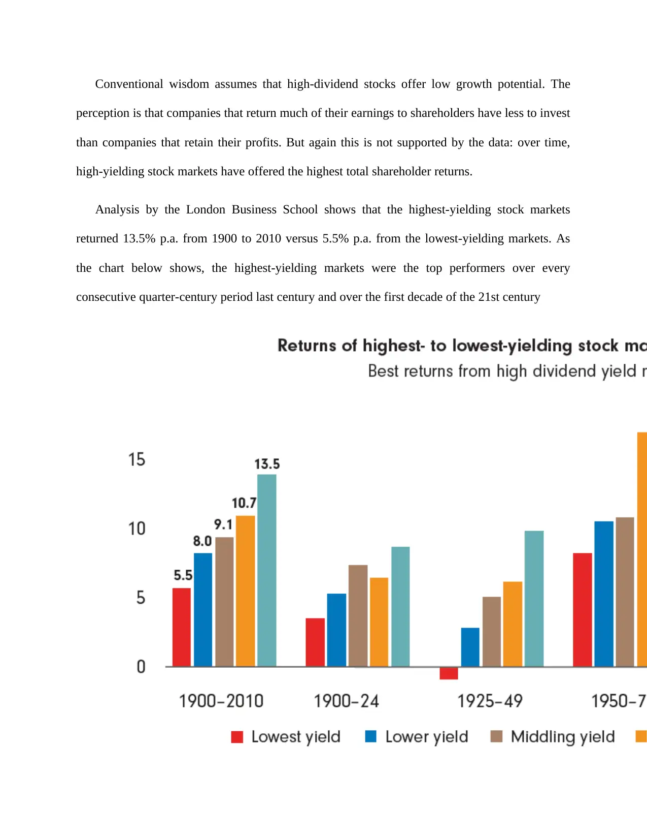
Conventional wisdom assumes that high-dividend stocks offer low growth potential. The
perception is that companies that return much of their earnings to shareholders have less to invest
than companies that retain their profits. But again this is not supported by the data: over time,
high-yielding stock markets have offered the highest total shareholder returns.
Analysis by the London Business School shows that the highest-yielding stock markets
returned 13.5% p.a. from 1900 to 2010 versus 5.5% p.a. from the lowest-yielding markets. As
the chart below shows, the highest-yielding markets were the top performers over every
consecutive quarter-century period last century and over the first decade of the 21st century

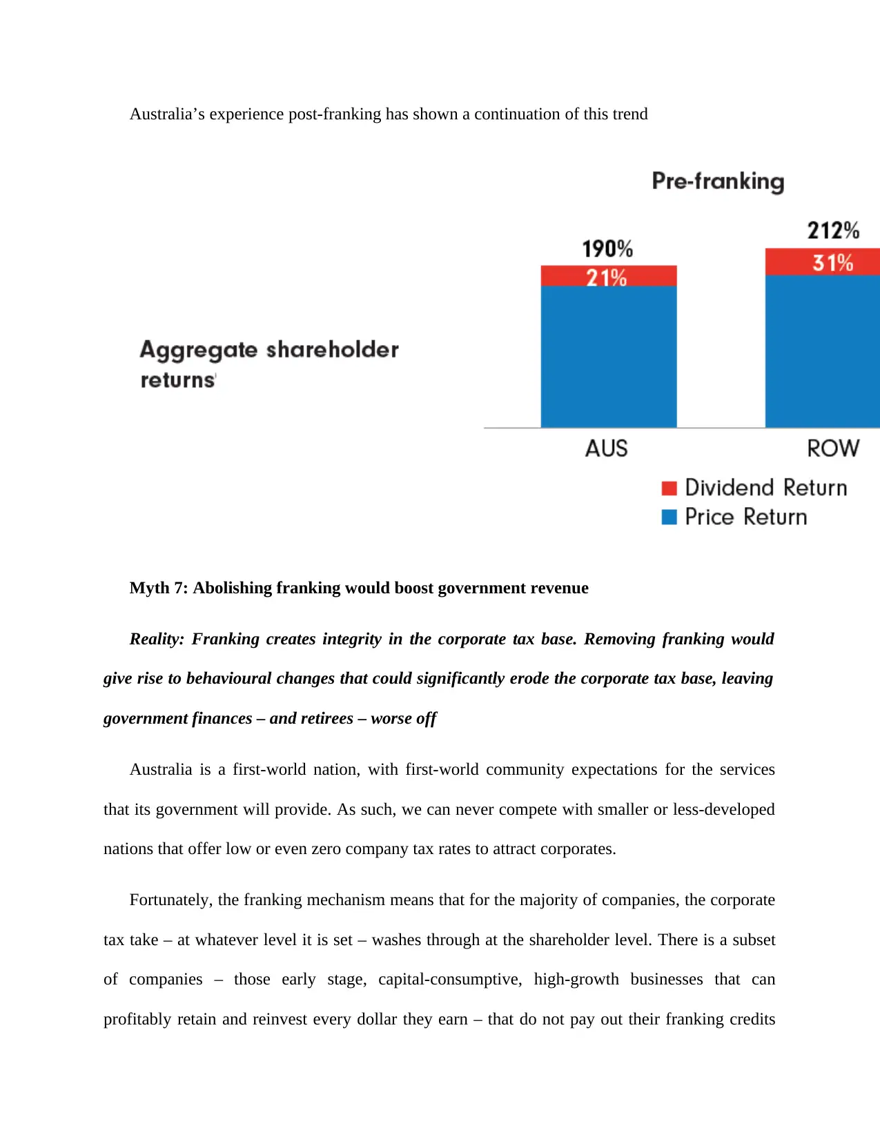
Australia’s experience post-franking has shown a continuation of this trend
Myth 7: Abolishing franking would boost government revenue
Reality: Franking creates integrity in the corporate tax base. Removing franking would
give rise to behavioural changes that could significantly erode the corporate tax base, leaving
government finances – and retirees – worse off
Australia is a first-world nation, with first-world community expectations for the services
that its government will provide. As such, we can never compete with smaller or less-developed
nations that offer low or even zero company tax rates to attract corporates.
Fortunately, the franking mechanism means that for the majority of companies, the corporate
tax take – at whatever level it is set – washes through at the shareholder level. There is a subset
of companies – those early stage, capital-consumptive, high-growth businesses that can
profitably retain and reinvest every dollar they earn – that do not pay out their franking credits

and thus would prefer a lower corporate tax rate. In theory, the risk is that these companies will
relocate to a more favourable tax locale. But tax is not the sole variable. We must ensure that
other policy settings (R&D tax settings, labour market flexibility, immigration flexibility, low
bureaucratic “red tape”, etc.) work together to make the Australian community a great place to
start – and grow – a business.
So a lower corporate tax rate could, at the margin, benefit and retain more of these mid-sized
growth businesses. However, there is a different and very significant risk that must be taken into
account. On a direct peer-group comparison basis, overseas companies exhibit more “lazy cash”.
Intuitively, we suspect this is related to their reluctance to repatriate cash earned outside of the
US into the US tax system.

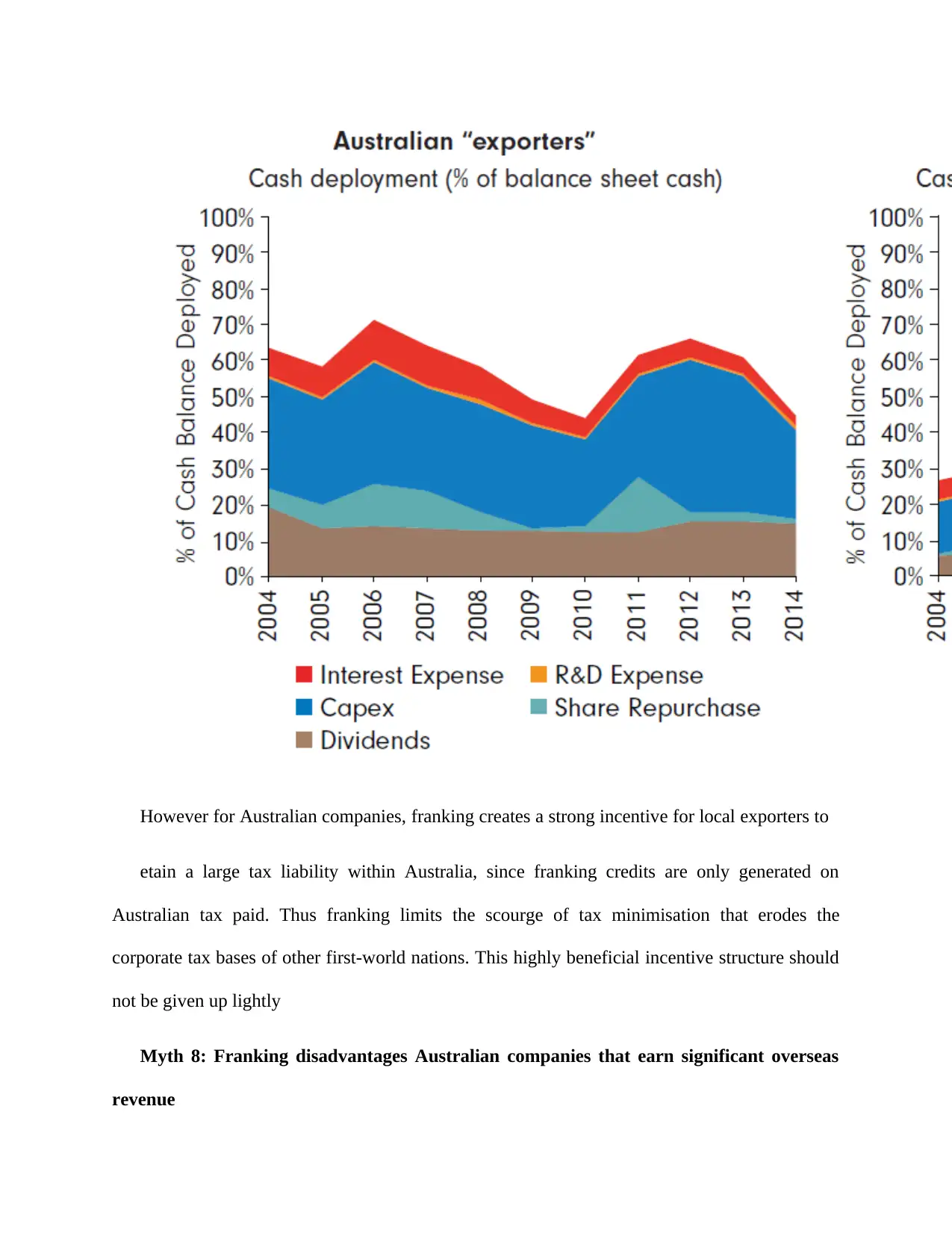
However for Australian companies, franking creates a strong incentive for local exporters to
etain a large tax liability within Australia, since franking credits are only generated on
Australian tax paid. Thus franking limits the scourge of tax minimisation that erodes the
corporate tax bases of other first-world nations. This highly beneficial incentive structure should
not be given up lightly
Myth 8: Franking disadvantages Australian companies that earn significant overseas
revenue

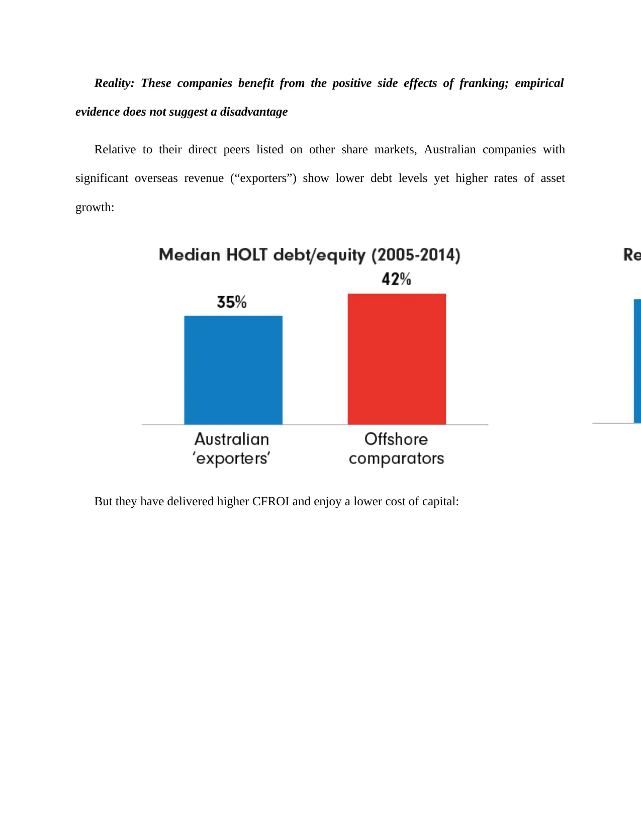
Reality: These companies benefit from the positive side effects of franking; empirical
evidence does not suggest a disadvantage
Relative to their direct peers listed on other share markets, Australian companies with
significant overseas revenue (“exporters”) show lower debt levels yet higher rates of asset
growth:
But they have delivered higher CFROI and enjoy a lower cost of capital:

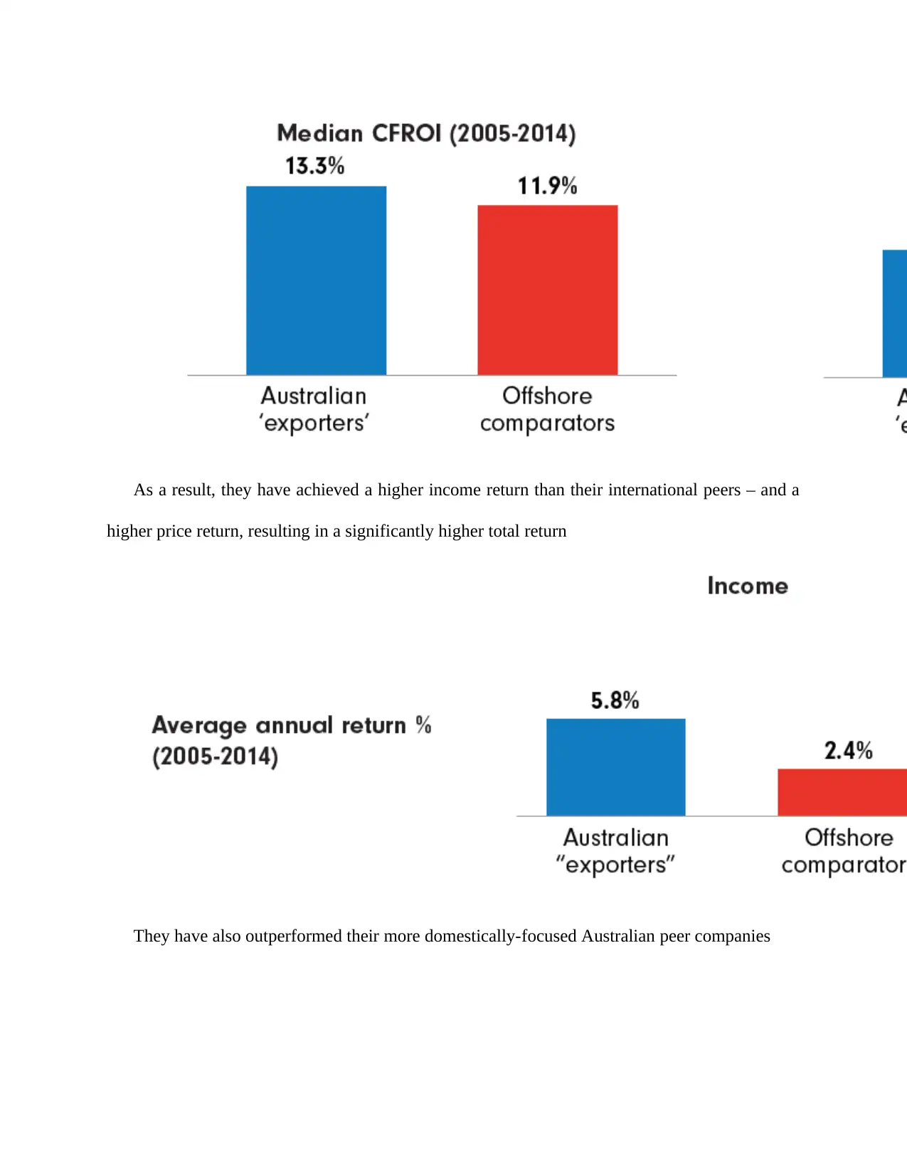
As a result, they have achieved a higher income return than their international peers – and a
higher price return, resulting in a significantly higher total return
They have also outperformed their more domestically-focused Australian peer companies

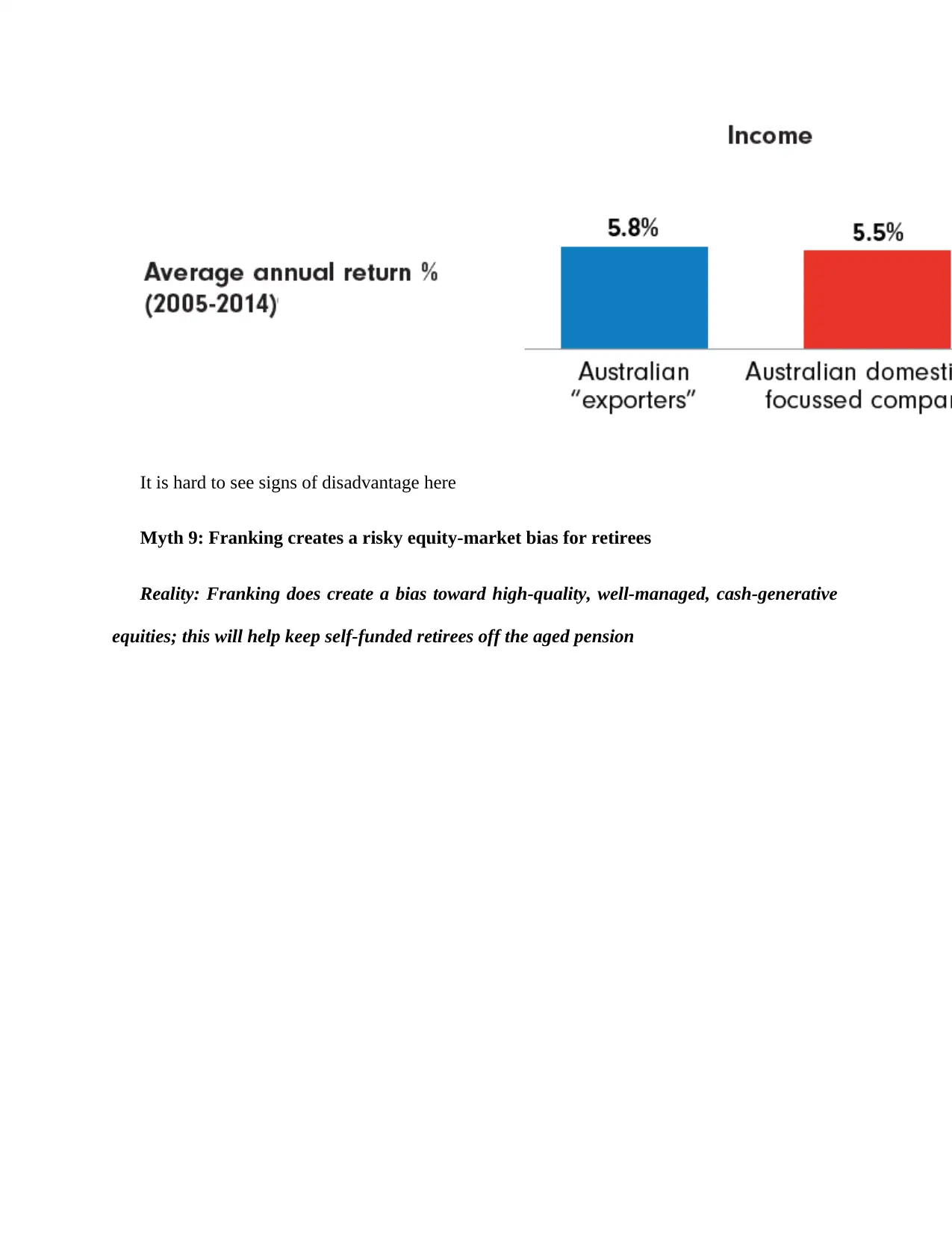
It is hard to see signs of disadvantage here
Myth 9: Franking creates a risky equity-market bias for retirees
Reality: Franking does create a bias toward high-quality, well-managed, cash-generative
equities; this will help keep self-funded retirees off the aged pension

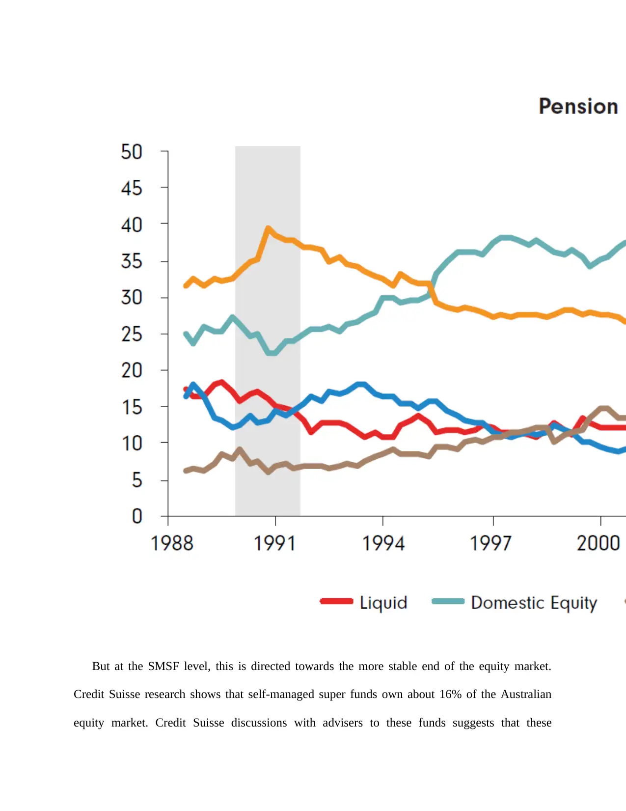
But at the SMSF level, this is directed towards the more stable end of the equity market.
Credit Suisse research shows that self-managed super funds own about 16% of the Australian
equity market. Credit Suisse discussions with advisers to these funds suggests that these

investors want high-dividend yields from large companies they identify with and have a history
of dividend growth. They have a Tier-1 group of stocks that includes the big four banks and
Telstra. The equity-ownership incentive created by franking does not prompt investment at the
speculative end of the market, which lessens the risk of retirees experiencing permanent loss of
capital. This exposure to quality, cash-generative growth assets is likely to help retirees maintain
their purchasing power throughout an extended retirement, and avoid falling back on the aged
pension
Myth 10: Franking creates a risky home-market bias for retirees
Reality: Franking results in well-managed, high-returning, lower-volatility companies that
are justifiably attractive to domestic and international investors
Franking constrains the reinvestment behaviour of Australian companies. This results in
leaner balance sheets, higher returns and lower volatility of returns. They are acutely aware of
the importance of maintaining sound balance sheets and of achieving high returns not just fast
growth. On the back of this – and deservedly for other reasons – Australian companies have
developed a reputation for being well-managed.
As a result of this, Australian companies are favoured by international institutional investors,
not just local retirees. This is evidenced by the cost of capital enjoyed by Australian companies,
which is in line with that experienced by US companies

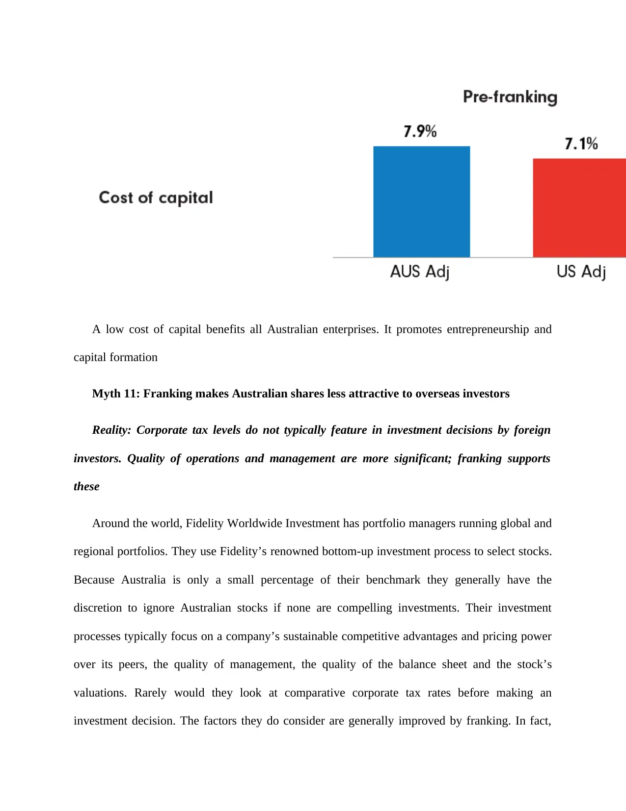
A low cost of capital benefits all Australian enterprises. It promotes entrepreneurship and
capital formation
Myth 11: Franking makes Australian shares less attractive to overseas investors
Reality: Corporate tax levels do not typically feature in investment decisions by foreign
investors. Quality of operations and management are more significant; franking supports
these
Around the world, Fidelity Worldwide Investment has portfolio managers running global and
regional portfolios. They use Fidelity’s renowned bottom-up investment process to select stocks.
Because Australia is only a small percentage of their benchmark they generally have the
discretion to ignore Australian stocks if none are compelling investments. Their investment
processes typically focus on a company’s sustainable competitive advantages and pricing power
over its peers, the quality of management, the quality of the balance sheet and the stock’s
valuations. Rarely would they look at comparative corporate tax rates before making an
investment decision. The factors they do consider are generally improved by franking. In fact,

because of tax certainty due to zero withholding tax on franked dividends, franking is actually a
simplifying factor for overseas investors. Perhaps the only time that tax would come into
consideration would be if a new tax, such as the recently proposed mining tax, was imminent or
corporate tax levels were to rise to a large extent. Australia’s dividend imputation system is a
non-issue for global equity investors.
3. Franking Credits – An all-inclusive overview
The process of investing undergoes a prior deep research based on fundamental analysis,
technical evaluation and macro-scenario analysis. But the concept does not end with the investor
risking his money on a lucrative stock. The most interesting part comes post investing, or after
the risk has been taken- the consequences. The fundamental rationale behind investing in equity
market is to earn profits and source out a stable form of income, and this happens through capital
appreciation as well as dividends.
Talking about dividends, we often come across corporate updates wherein the company has
offered franked dividends for quarterly/semi-annually/annually basis. Today, Material sector
player, Amcor PLC (ASX: AMC) has announced an unfranked quarterly dividend of AU
0.17725 cents per share. Iron ore giant, BHP recently announced fully franked final dividend of
US 78 cents/share. Several other companies have updated the market with their dividend payout
plans in the ongoing reporting season.
Today’s article would provide you with a holistic understanding of one of the dividend
constituents- Franking Credits. Let us dive right in:

Understanding Franking Credits
Often synonymously used as imputation credit, franking credit could be best described as the
type of tax credit which is paid to the shareholders by the company they would have invested in,
along with the dividend payments.
Franking credits could exist as a consequence of an entitlement to a franked distribution, when
the company is a beneficiary of a trust. The concept is fairly famous in Australia, with several
companies offering franking credits to eliminate or at least reduce any sort of double taxation,
depending on the investor’s tax bracket. Shareholders avail a reduction in their income taxes or
are granted a tax refund, as the company distributing the dividend, already pays the tax on them
and the franking credit allows the company to allocate a tax credit to their shareholders. In the
Australian context, a franking credit can be described as an entitlement, offered to the
shareholders by a company they would have invested in, to a reduction in personal income tax
which is payable to the Australian Taxation Office.
Australia, New Zealand and Malta have imputation systems, whereas countries like the UK,
Chile, Korea and Canada have a partial imputation system.
Breaking Down The Concept

Often, you would have come across the term ‘franked’ when it comes to dividend distribution.
Dividends are paid out of the generated profits subject to the Australian Company Tax system,
which means that the shareholders are granted a rebate for the tax which is paid by the company
on the profits that are distributed in the form of dividends.
Let us take an example: Mr X is the owner of shares in a company, that pays him a fully franked
dividend of $800. The dividend statement states that a franking credit of $200 exists,
representing the tax amount on the dividend which the company would have paid. When Mr X
declares his personal income, he would state an amount of $1000, (which was the actual
dividend). If the tax rate was 15%, he would have paid $150 tax on the dividend, but as the
company has already paid the franking credit amount as tax, Mr X would receive a refund of
$50. In case Mr X was on a higher tax slab, he would not be entitled to avail a refund, rather he
would be paying extra tax. On the contrary, a lower bracket slab would lead to the possibility of
full refund.
History of Franking Credits
The concept of franking credits was brought into consideration in the late 1980s by the Hawke
Government, making it a relatively new area in the business line. The franking credit imputation
system has existed in Australia and its taxation system for approximately 30 years. In the
beginning, the franking credit system was granted exclusively for the offsets on the tax amount
paid. This was modified in 2001, which allowed the cash refund of the excess credits to
shareholders who had their tax liabilities lower than the refunded credits.

Benefits of Franking Credits
The concept, even though is new, has proven its advantages for both companies and
shareholders. Some of these are mentioned below:
Calculation of Franking Credits
In Australia, in order to be eligible to receive franking credits, one needs to hold their shares for
over 45 days at risk, which is the 45 day Holding Rule. The franking credit to be paid to a
shareholder can be derived using the following formula:
Functionality of Franking Credits

The franking credit is attached to a dividend which the company pays to shareholders out of its
after-tax profits. Its worth is the same as the amount of tax which is paid on the individual’s
share from the profit generated by the company, before it was distributed as a dividend. Intended
to shun down or remove the double taxation concept, because the tax on dividends is already
been paid by the company, when personal income tax is computed for the individual, the value of
their accrued franking credits can be subtracted from the tax payable.
A company can differ from the another in the way that it deals with franking credits, depending
upon the amount of tax they have paid. It should be noted here that the company cannot offer a
franking credit exceeding an amount that is paid in company tax, and they cannot offer the
franking credit for tax that has been paid in a foreign country. In the context of Australia, this
means that the benefit of franking credit is exclusively available to Aussie residents and cannot
be claimed by the foreign proprietors of the Aussie companies.
Franking Credits On The ASX
As per a report from the Australian Securities Exchange, in the S&P/ASX 200 index, which
marks the 200 biggest players of the Australian equity market, 184 companies had paid
dividends in the 52 weeks to 19 April 2018. Of these companies, half granted fully franked
dividends and around a fourth paid semi-franked dividends and unfranked dividends. The highest
franking balances on the market included (in no particular order) Commonwealth Bank of
Australia (ASX: CBA), BHP Billiton Limited (ASX: BHP), Westpac Banking Corporation
(ASX: WBC), Woolworths Group Limited (ASX: WOW) and TPG telecom Limited (ASX:
TPM).
Key Takeaways:

 Imputation credit or franking credit is the type of tax credit which is paid to the
shareholders by the company along with the dividend payments to avoid double taxation.
 The concept of franking credits was brought into consideration in the late 1980s by the
Hawke Government
 In Australia, in order to be eligible to receive franking credits, one needs to hold their
shares at risk for over 45 days at risk, which is the ‘45 day Holding Rule’.
 A company cannot offer a franking credit exceeding an amount that is paid in company
tax, and they cannot offer the franking credit for tax that has been paid in a foreign
country.
4. Labor's tax policies 'highly progressive' with top 20% feeling most impact
A new analysis of Labor’s tax policies says the proposed overhaul of franking credits,
changes to negative gearing, trusts and capital gains tax if Bill Shorten wins the election on
18 May will have a negligible impact on the bottom 50% of households in Australia
measured by income and wealth.
While the Morrison government has played up the negative impact of revenue measures,
particularly franking credits, on self-funded retirees with modest incomes, the distributional
analysis of Labor’s tax measures by the Australian National University’s Centre for Social
Research and Methods says that’s largely bunkum.

“Franking credits benefit households in the top 20% of income and wealth distribution
considerably more than other households,” the analysis says. “While these households often
have low taxable incomes, they tend to have large wealth balances or be in households with
high incomes, even when the individual affected has a low income.”
The ANU academics, led by economic and social researcher Ben Phillips, modelled Labor’s
changes to dividend imputation, negative gearing and capital gains tax, the reinstatement of
the budget levy, the low and middle-income tax offset, new personal income tax rates and
thresholds, and the taxation of trusts.
The overall impact of the proposed changes was highly progressive, “with virtually no
impact for households in the bottom 40% of the income distribution and the largest increase
for those in the top 10%”.
“In raw dollar terms, the top 20% account for around 70% of the fiscal impact with a loss of
disposable income of around $17bn out of around $25bn in increased revenue under Labor.”
The ANU analysis says the top income decile will see an average loss of disposable income
of $11,877 per year under Labor compared with the 2019 budget handed down by the
Morrison government just prior to the election – which compares to reduction in income for
the bottom five deciles of below 1%.

On franking credits, the analysis says the largest impact in dollar terms and as a percentage
of disposable income of Labor’s policy falls on the top 10%.
The top 10% would, on average, pay $2,641 a year, or 1.1% of disposable income, if Labor
wins and franking credits are removed. It says there is “virtually no impact” on low income
groups in the bottom half of the income distribution. It says 600,000 households are
negatively affected by the removal of franking credits.
The study also indicates Labor will have room to move fiscally to increase the Newstart
allowance by $75 per week for singles, at a cost of around $3bn per year.
The new ANU analysis comes as the shadow treasurer, Chris Bowen, accused “vested
interests” of attempting to influence the election outcome, taking aim at the Real Estate
Institute of Australia for campaigning against proposed negative gearing and capital gains tax
changes.
REIA has boasted that its campaign, assisted by its network of real estate agents, has reached
nearly 8 million Australians.

Campaign catchup 2019: leaders on the home straight
Read more
“This is part of a concerted effort by a select group of property interest groups to decide an
election outcome and Australians should be alive to it,” Bowen said. “The REIA’s
irresponsible claims are just downright lies.
“Labor’s housing affordability reforms will our first home buyers on a level playing field
with property investors and importantly, give renters saving for their first home a chance.”
In a letter sent to tenants, REIA warns that “rents will go up” under Labor’s policy.
“Because you’re currently renting, it might be tempting to dismiss the latest political battle
over whether negative gearing should be abolished. You might even see it as a good thing if
house prices go down, but rents will rise”.
5. If franking credits and negative gearing didn’t exist, no one would invent them

abor’s plans to unwind refundable franking credits and negative gearing are the most
controversial tax changes taken to an election since John Howard’s GST two decades
ago. There’s plenty of opposition from retirees on yachts pointing to the
thousands of dollars they’ll lose in franking credits, and the property lobby is warning
of a housing crash if negative gearing is changed.
But let’s think about it another way. Imagine that refundable franking credits and
negative gearing didn’t exist, and instead the Coalition was promising to introduce
them. How might the debate be different?
First, instead of simply pointing to people who lose from their removal, the
Coalition would have to explain why these policies should exist in the first place.
That’s a much harder ask.
The Coalition would no doubt rely on some standard tax policy principles. The basic
principle of franking credits is that company tax is simply paid on behalf of
shareholders, at each shareholder’s marginal personal income tax rate. And so any
unused franking credits are in effect an overpayment of prepaid tax, and should be
returned via a cheque from the government.
In addition, it would point to the unfairness of retirees in self-managed super funds
being denied (non-refundable) franking credits, whereas retirees in industry and retail
super funds can get the benefits because their credits can be used to offset the tax of
younger members who are taxed on their contributions and fund earnings.
In arguing for negative gearing, the Coalition would presumably point to the standard
principle that losses should be offset against income before it’s taxed. Tax
experts would quibble that any losses would be deducted in full, while only half
the capital gains are taxed.
But such arguments from principle are rarely enough to win a tax debate. Theoretical
purity is all well and good, but there are plenty of other considerations that take into
account how things work out in practice. And here the case would become much
harder to make.

Retirees might question why the government should send cheques for $6 billion a
year to the wealthiest Australians, instead of doing more to help pensioners,
especially renters, at risk of poverty and financial stress in retirement.
After all, more than half the benefits of refundable franking credits for self-managed
super funds go to funds with balances of $2.4 million or more. And shareholdings
among over-sixty-fives outside super are also highly skewed towards the wealthy: the
richest 20 per cent of households over sixty-five own 86 per cent of the shares held
directly, while the poorest half of all retirees own less than 2 per cent.
Others would question whether the budget can afford such giveaways, especially
when fifteen years of intergenerational reports have warned us of the long-term
budgetary threat from the ageing of the population. Are refundable franking credits
really appropriate when fewer than one in six retirees pay any income tax?
Are they affordable if they lead to the average retired household with $100,000 in
income a year paying the same amount of tax as a working household earning
$50,000?
With negative gearing, we’d be debating whether it’s really a priority to spend
between $1 billion and $2 billion a year of taxpayers’ money on tax breaks for
housing investors, especially when most investors would simply purchase existing
properties. Voters might also be worried by projections showing that negative gearing
would push down home ownership as negatively geared investors outbid first
homebuyers at auctions.
And how would the public weigh these policies compared with their alternatives?
The $6 billion annual savings on refundable franking credits would be enough to fund
a 40 per cent increase in Commonwealth Rent Assistance for all
income-support recipients ($1.2 billion) and relax the taper rate on the age
pension assets test ($750 million a year), with plenty left over to shore up the budget
against the long-term costs of an ageing population.
And if we’re serious about boosting housing construction, $1 billion in incentive
payments to state governments to reform land-use planning rules and get

more housing built in the inner and middle suburbs of our major cities would be far
more effective.
Of course, the big difference between this imagined world and real life is that we
wouldn’t have a cacophony of special interest groups arguing so loudly to keep
refundable franking credits and negative gearing.
People prefer what they know, and like keeping what they have. These biases are
powerful allies for those defending bad policies. Take them away, and the case for
change becomes clearer.
The reality is that no major party would be able to defend introducing these policies
today. And if you can’t make that case, we should worry less about abolishing them. •
6. Do Franking Credits Matter? Exploring the Financial Implications of Dividend
Imputation
1. Executive Summary Questions have been raised over the efficacy of the dividend imputation
system, including by the Financial System Inquiry in November 2014 and the Tax Discussion
Paper released on 30 March, 2015. We aim to contribute to the policy debate by examining the
financial implications of the imputation system for markets, companies and investors. We
address the impact of dividend imputation for stock prices and returns, cost of capital, project
evaluation, capital structure, payout policy and investor portfolios. We also discuss potential
impacts if the imputation system was dismantled or adjusted, perhaps in conjunction with a
reduction in the corporate tax rate. This report draws on the literature and available evidence to
identify the issues, and offer some novel perspectives. Key Findings 1. The effects of imputation
are debatable both in theory and practice along most dimensions. The implications of imputation
for stock prices and returns, cost of capital, capital structure and investor portfolios are all
unclear. The notable exception is payout policy, where higher payout ratios have clearly been
encouraged by the desire to distribute imputation credits. 2. Whether imputation is priced into the

market is a central issue. Unfortunately, both theory and evidence provide very mixed
indications, and there is no consensus. The effects of imputation can be seen in share price
movements around dividend events, but are not readily apparent in returns or price levels.
Against this mixed evidence, the Tax Discussion Paper stance that the cost of capital is set in
international markets stands as an extreme position. Allowance should be made for the
possibility that imputation might be priced partially, or even fully, in some situations. 3. One
area where imputation probably matters is small, domestic companies. It is the smaller, domestic
segment where it is more likely that local investors who value imputation credits may determine
prices, as well as being chiefly responsible for providing funding. Any adverse impact from
removing imputation may well be concentrated in this (economically significant) segment. 4.
How imputation influences behaviour is important. Focusing on how imputation impacts on
precise computations like cost of capital estimates is arguably less important than understanding
the behaviours that imputation encourages, and how these might change if the imputation system
was adjusted. Investors and company management often do not formally build the value of
imputation into share price valuations, cost of capital estimates, or evaluations of investment
projects. Nevertheless, these players may still acknowledge that imputation credits are valuable
to many shareholders, and behave accordingly. Imputation can thus have an important influence
on some decisions, even though it may not be explicitly incorporated into any supportive
analysis. 5. The relation between imputation and payout policy deserves attention. The
contribution of the imputation system to lifting payout ratios has arguably been one of its key
effects and main benefits. By encouraging greater payouts, and thus requiring companies to
justify their case when seeking additional funding, the imputation system has probably
contributed to more disciplined use of capital. From this perspective, dismantling the imputation

system could have detrimental effects for both shareholders and the Australian economy through
less efficient deployment of capital. 6. Imputation may not have much impact on corporate
capital structure or investment decisions. The link between imputation and both capital structure
and project evaluation is tenuous. The case is stronger for a relation with capital structure, given
that imputation increases the net return available to many shareholders. However, linking
imputation to capital structure requires companies to be concerned with personal tax effects
when making funding decisions; which are www.cifr.edu.au Page 4 one of many potential
influences on capital structure identified in the literature. When estimating cost of capital and
evaluating projects, the evidence suggests that few companies take imputation into account.
Rather, corporate investment decisions appear primarily based on more subjective
considerations, with financial analysis providing a supportive role. 7. Imputation is influential in
regulatory decisions. Regulation of utilities is one area where the value of imputation is
explicitly built into the computations, and has real effects in terms of output prices. The impact
of changes in imputation on utility prices should be given specific consideration in
contemplating any policy changes. 8. The influence of imputation on investor portfolios is
unclear; but any resulting domestic bias should not be a major policy concern. Home bias is
observed everywhere around the world, and has many potential explanations. The degree of
home bias among Australian investors does not seem untoward, except perhaps in the Self-
Managed Superannuation Fund sector. Further, just because a portfolio fails to reflect the
available asset universe does not necessarily mean that it is exposed to significant and
unwarranted non-diversifiable risk: the bulk of diversification opportunities can be secured with
a just a few assets. We see no significant danger to the Australian economy or financial system
from having a bias towards Australian equities paying high fullyfranked dividends. In any case,

it is doubtful that this bias could be substantially addressed through changes to the imputation
system. 9. The potential effects from removing or adjusting the imputation system are
conditional on what else happens. Many of the potential effects from changing the imputation
system depend on what other tax changes occur. Most relevant is any concurrent reduction in the
corporate tax rate, which might provide a full or partial offset in some areas. Whether the
corporate tax rate is changed could be particularly important for the tenor of any share price
reaction, and any encouragement to change capital structure. A major exception is payout policy,
where reducing the availability of imputation credits would dull the incentive to distribute
earnings regardless. We note that the impact on investment from a reduced corporate tax rate
may be diluted to the extent that tax effects and cost of capital are second-order influences on
investment decisions. This paper proceeds as follows. Section 2 provides background on
dividend imputation and the related policy debate. Sections 3 and 4 examine the theory and
evidence on how imputation manifests in stock prices, expected returns, and thus cost of capital.
Section 5 describes how imputation reflects in cost of capital estimates and project evaluation in
practice. Section 6 considers the link between imputation and capital structure; while Section 7
addresses payout policy. Section 8 discusses how imputation impacts on investor portfolios,
including any notable clientele effects. Section 9 concludes. 2. Background We commence by
providing historical context on Australia’s imputation system. This is followed by an overview
of the Tax Discussion Paper, including evaluation of the framework under which it was prepared.
We also discuss the potential scope of changes that might occur to the imputation system. 2.1.
Historical Context The imputation tax system is not the modern development of the Australian
tax system that many believe. Rather, it is the so-called classical tax system that is the relative
newcomer. Under a classical system, corporate profits are taxed both at the corporate level, and

again upon distribution of dividends to shareholders, which are taxed at the latter’s marginal
income tax rate. Under an imputation system www.cifr.edu.au Page 5 investors are only taxed at
their personal income tax rate on dividends and get a full, or partial, rebate of taxes paid by the
company. Income taxes were introduced in Australia by the States towards the end of the
nineteenth century. By the end of that century, several States had imposed a tax on the dividends
that companies paid. However, the dividends were then exempt from tax when received by the
shareholder. When the Commonwealth began taxing companies in 1915, only undistributed
profits were taxed, and dividends were taxed only in the hands of shareholders. By 1923,
companies became taxable on all their profits. While shareholders were liable for taxes on
dividends received, they received a rebate for the company tax that had been paid. This persisted
until 1940, when the tax rebate was abolished (see Livingstone, 1977). It was at this point that
Australia moved to a classical tax system. The situation was reversed for Australian residents on
1 July 1987, when a full imputation system replaced the classical taxation system. As
Livingstone (1977) points out, fundamental to the classical tax system is an entity viewpoint,
while fundamental to the imputation system is an ownership viewpoint. Livingstone also points
out that the choices made by governments about tax systems have largely been driven by
pragmatic considerations regarding revenue, e.g. in Australia’s case, the need to fund
participation in two World Wars. A number of changes were subsequently made to the
imputation system, two of which are most notable for our purposes: • 1 July 1997 – The ‘holding
period rule’ was introduced, which required investors to continue holding1 a stock for 45 days
about the ex-dividend date in order to claim the imputation credit. This was intended to prevent
various arbitrage schemes and indirect trading of imputation credits, hence blocking an avenue
for foreign (and tax-exempt) investors to extract value from imputation. • 1 July 2000 – The

‘rebate provision’ was introduced, making imputation credits fully refundable. This made a tax
refund available where credits exceed other tax liabilities, thus enhancing the value of imputation
to low or zero tax resident payers such as superannuation funds, charities and retirees. The
research into imputation is extensive in some areas, and somewhat thinner in others. Initial
research around the time that imputation was introduced tended to have a ‘policy’ focus and was
aimed at understanding the economic implications of imputation, with involvement from
government bodies such as the Australian Commonwealth Treasury and the Reserve Bank of
Australia. Some years after the introduction of imputation, an active agenda emerged in the
finance literature examining the implications for share prices, cost of capital and (to a lesser
extent) corporate finance policy. Academic research in these areas has remained active since, in
part spurred by the relevance of imputation for utility regulation. One of the key tasks undertaken
in this paper is to provide an overview and synthesis of this body of research. Interest in
imputation from a public policy perspective has been renewed in recent years, exemplified by the
Henry Tax Review released in 2010 (Henry, 2009) and the recent Tax Discussion Paper (TDP)
of 2015. The value of the imputation system was also queried by the Financial System Inquiry of
2014. Much of the recent public policy debate is focused around whether Australia would be
better off adjusting or even removing the imputation system, and using the revenue increase to
fund a reduction in the corporate tax rate, thus moving back towards a classical tax system. The
case for doing so was 1 Investors are also required to remain exposed to the risk of price
fluctuations.
Interest in imputation from a public policy perspective has been renewed in recent years,
exemplified by the Henry Tax Review released in 2010 (Henry, 2009) and the recent Tax
Discussion Paper (TDP) of 2015. The value of the imputation system was also queried by the

Financial System Inquiry of 2014. Much of the recent public policy debate is focused around
whether Australia would be better off adjusting or even removing the imputation system, and
using the revenue increase to fund a reduction in the corporate tax rate, thus moving back
towards a classical tax system. The case for doing so was 1 Investors are also required to
remain exposed to the risk of price fluctuations, but can hedge that exposure to a delta of 0.7.
Other concessions were made for small investors, and for institutional investors tracking an
index. Such concessions, coupled with a two year legislative delay, resulted in a rather weak
restriction on arbitrage in the early years of the 45 day rule. www.cifr.edu.au Page 6 put
forward in an influential CEDA paper prepared by David Gruen in 2006 (Gruen, 2006). We
sketch out and evaluate the discussion appearing in the TDP in the next sub-section. 2.2. The
Tax Discussion Paper (TDP) The TDP raises the question of whether Australia is getting
value out of its imputation system. For context, we list below the relevant aspects mentioned
in “Section 5: General Business Tax Issues”, followed by discussion of the conceptual
underpinnings of the TDP’s stance. The TDP makes the following points: On company tax: •
The Australian corporate tax rate, and the ratio of corporate tax to total tax revenue, are
relatively high in a global context. • The economic burden of corporate tax is shared among
shareholders, consumers and employees. • Corporate tax detracts from the return on
investment. In turn, this “reduces the level of investment in small, open, capital importing
economies, such as Australia … because the marginal investor in Australia is likely to be a
non-resident, who will invest … only if they achieve an after-tax return that matches their
target rate of return” (page 78). The TDP effectively argues that a higher corporate tax rate
boosts the required pre-tax return, which leads to lower investment by foreigners; and infers
that this is detrimental to all Australians. • Higher corporate tax rates increase the incentive

for foreign investment to be funded by debt, which may erode the Australian corporate tax
base. On the benefits of imputation: • Imputation provides strong incentives for Australian-
owned companies to pay tax in Australia, i.e. it has integrity benefits for the tax collection
system. • It is acknowledged that imputation increases the rate of return for Australia
investors; but this is noted in the context that the associated company tax meanwhile pushes
up the pre-tax return that is required to attract non-resident shareholders. Effectively,
Australian investors earn a bonus over the market-clearing rate of return, as determined in
international capital markets. • Through encouraging greater use of equity financing,
imputation may improve economic stability. On the costs of imputation: • Imputation reduces
government revenue, with around $19 billion p.a. of imputation credits claimed over recent
years. Revenue concerns related to the refundability of imputation credits for low or zero tax-
payers ($4.6 billion in 2012-3) also receive a specific mention. • The biases created by
imputation may be undesirable in an increasingly open and globalised world. • Imputation
“does not help attract new investment into Australia” (p87); an argument that the TDP links
to the effects of the higher required returns stemming from the corporate tax rate (see above).
• Imputation reduces the effectiveness of tax concessions, such as for research and
development. • Imputation adds to the complexity of the tax system. Other effects from
imputation (with no comment on whether they are beneficial or detrimental): • Australian
investors have an incentive to invest more in Australian shares. • Imputation creates a bias
against Australian companies investing overseas. • Imputation creates a bias towards
distributing earnings as dividends, rather than retention. www.cifr.edu.au Page 7 The
conceptual underpinnings running through the TDP largely arise from the economics
literature on tax incidence in an international context (for reviews, see: Auerbach, 2005;

Griffith, Hines and Sørensen, 2010). A key assumption is that Australia is a small, open
economy that has no control over required returns, which are set at the margin in
international capital markets. This equates to the proposition that imputation does not lower
the cost of capital, and has no influence on the ‘hurdle rate’ of return that a company is
required to deliver (after corporate tax, but prior to investor taxes). The underlying
assumption is that assets are entirely priced by an international marginal investor who places
little or no value on imputation credits. A major contribution of this report is to examine the
evidence for this proposition arising from the finance literature. As it will be seen, whether
imputation is ‘priced’ and hence impacts the cost of capital remains the subject of much
debate. Accordingly, the validity of the core assumption that required returns and cost of
capital are set by international investors cannot be taken as given; and is an extreme position
along the spectrum of possibilities. Indeed, whether prices are set by a marginal investor, or
by aggregation across investors, is an open question (discussed in Section 3.2). It is our
contention, therefore, that a policy decision should not be based on the assertion that the
marginal investor setting prices in the Australian market is an overseas investor. To do so
would base policy on an insecure foundation, and risks serious error. A notable sub-text in
the TDP’s stance is that higher corporate tax rates reduce economic prosperity for Australia
through diminishing foreign investment; and that the incidence of a high corporate tax rate is
ultimately borne by Australian consumers and employees as a consequence. The mechanism
involves a higher corporate tax rate acting to increase the required return, which results in a
reduction in foreign investment, which in turn leads to lower economic growth and
employment. It is not our main intent to comment on the corporate tax rate per se.
Nevertheless, it is clear that the TDP links the rationale for reconsidering imputation to the

presumption that it has failed to reduce the cost of capital because international investors do
not benefit. It is implied that a revenue-neutral shift involving a lower corporate tax rate
funded by a removal of imputation can lead to a lower cost of capital, higher investment, and
hence greater economic prosperity. This is essentially the line adopted by Gruen (2006), who
appeals to applying higher taxes on immobile factors such as wages along with lower taxes
on mobile factors like capital, following Ramsay (1927). The TDP stance on the effects of
reducing the corporate tax rate may also be questioned on a number of fronts. For instance,
the potential for investment to increase may be attenuated by the effects of less mobile
capital, 2 or complex interactions between tax and risk. There are also some difficult
implementation issues to consider. Reducing the corporate tax rate may induce tax leakage
from personal taxes as the tax rate gap widens. Lowering taxes on foreign companies (while
removing imputation for locals) might be politically unpalatable. An overview of most of
these issues can be found in Auerbach (2005), Griffith, Hines and Sørensen (2010), and
Sørensen (2014). A further notable sub-text is that the TDP (and the Financial System
Inquiry) queries the value of imputation in light of increasing globalisation. While the trend
towards increasing globalisation is evident, the extent to which financial markets are
integrated remains an open question. The evidence seems to point towards partial integration,
with smaller niches such as emerging markets often remaining largely driven by local forces
(see Lewis, 2011). Consistent with this notion, Durand, Limkriangkrai and Smith (2006) find
that returns on larger Australian stocks appear to be explained by US factors, while the same
does not hold for Australian small stocks, which appear to be priced locally. This leaves
some doubt over the extent to which integrated, global pricing applies. We discuss this issue
further below, including in Sections 3.2 and 8.1. 2 Capital mobility can be hampered due to

the existence of adjustment frictions, location-specific assets or rents, and smaller, local-
bound companies. www.cifr.edu.au Page 8 Overall, the picture is considerably more complex
and mixed than portrayed in the TDP (which is admittedly only a discussion paper, not a
statement of position). There is no doubt that there is an element of truth in the proposition
that funding a reduction in the corporate tax rate by removing imputation would attract more
foreign investment, which would enhance Australian economic growth in itself. However,
the ultimate effects are very unlikely to be either pure or unambiguous. There is considerable
scope for mitigating influences and unanticipated reactions. For instance, eliminating
imputation may have adverse impacts on locally-sourced investment; while tax changes can
lead to changes in behaviour that result in revenue losses that can be hard to anticipate (e.g.
substitution of declared corporate income for personal income; local companies shifting
overseas; possibly reduced capital gains tax). The extent to which tax is a first-order effect in
determining investment decisions is also debatable: we comment further on this issue in
Section 5.1. Having raised these broad issues, we leave it to others to contemplate them in
more depth. 2.3. Scope of Potential Changes to the Imputation System Both the TDP and the
Financial System Inquiry (2014) have called for a review of the imputation system, rather
than specifically requesting comment on its potential dismantling. Further, Treasurer Hockey
has stated that he is more interested in how the imputation system might “be improved”,
rather than “get rid of it” (Australian Financial Review, 13 April, 2015, p5). Interestingly, at
the time of writing, the lead article for The Economist analysing the problem of too much
debt, partly caused by the tax deductibility of debt interest, suggests: “The purest option is to
abolish corporate tax entirely and instead have one layer of tax levied on the income that
individuals receive from investments in firms”. 3 At least for dividends received by

Australian residents, this is what imputation achieves. The TDP observes that a wide variety
of tax treatments for dividends are used in other countries, including partial double taxation
systems where dividends are taxed at preferential rates, or where certain tax credits are made
available to ease the double taxation of corporate earnings. It lists only Australia, New
Zealand, Chile and Mexico as having full imputation systems; plus Canada as providing a tax
credit related to notional domestic corporate profits. The possibility exists that the imputation
system might be modified, or replaced with a close alternative. One option is removing the
rebate for excess imputation credits, which would largely impact zero tax-paying entities
such as charities and retirees. We will proceed by discussing a hypothetical scenario where
the imputation system is totally dismantled, both in isolation, and in parallel with a reduction
in the corporate tax rate. In the latter case, we base our analysis around a reduction in the
corporate tax rate from 30% to 20%, in accordance with Gruen (2006). Our aim is to
establish juxtapositions to the current full imputation system. Any changes would probably
sit somewhere between the two extremes. 3. Theory – Imputation, Share Pricing and the Cost
of Capital We start by discussing the theory and related issues regarding how imputation
manifests in share prices, required returns and hence the cost of capital. The underlying
principle is that share prices are set by the market to generate to a certain expected return or
‘required return’; which in turn establishes the cost of capital as the hurdle rate that a
company needs to deliver on its investments in order to generate economic value. The
fundamental question is really whether imputation affects company value. There is only one
value for a company, but many ways to measure its ‘cost of capital’. Whether imputation
changes the cost of capital depends on the definition used, including whether cost of capital
is measured before tax, after corporate tax, or after all taxes; and how imputation tax credits

are 3 “ The Great Distortion”, The Economist, 16 May 2015, 15-18 (see page 17).
www.cifr.edu.au Page 9 accounted for. For example, if an ‘after corporate tax cost of capital’
definition is used, and imputation credits are accounted for in cash flows when valuing the
company, then there is no imputation effect on the ‘cost of capital’ so defined. We recognise,
however, that much of the debate around imputation is couched in terms of the cost of
capital. This debate is typically focused on the after corporate tax cost of capital, with
imputation credits accounted for by adjusting cost of capital. Also relevant is the basic
economic distinction between ‘value in use’ and ‘value in exchange’. There is no doubt that
imputation credits have considerable value in use to Australian resident investors, who can
use them to reduce taxes. Whether they have value in exchange – in other words, whether
they are priced – is a separate matter. This fundamental issue can be posed as follows.
Consider two companies with identical assets, with the exception that one also has a positive
balance in its franking account and can distribute imputation credits, while the other has a
zero balance. The question is: “Do the two companies sell for the same price?" Against this
background, we will address three specific questions: • How do tax effects influence the
return required by various investors? We describe the theory and the issues that arise in
Section 3.1. • When the tax status of investors differs, how do tax effects manifest in
equilibrium share prices and required returns? This is the nub of the issue, and is
controversial. We outline the theoretical issues in Section 3.2, and detail the empirical
evidence in Section 4. • How is imputation taken into account when making decisions? To a
large extent this is an implementation issue, the evidence for which will be discussed with
respect to investors in Sections 4.3 and Section 8, and for companies through Sections 5 to 7.
However, this question cuts across agency theory and behavioural influences, which we

briefly acknowledge in Section 3.3. Our review raises plenty of issues, but yields no clear
direction on whether imputation credits should be priced from a theoretical perspective. 3.1.
Investor Taxes and Required Returns We commence by outlining how imputation and other
tax effects impact on the post-tax returns for various investors. This sets up a basis for the
discussion in Section 3.2 on the mechanism by which tax effects manifest in prices and
required returns in equilibrium, and henceforth ultimately determine the cost of capital for a
company. The relation between imputation and an investor’s required return is one
component within the broader issue of how tax effects manifest in asset prices and returns.
This topic has been widely studied, including how investor (personal) taxes and corporate
taxes interact to influence investor returns, and the associated implications for cost of capital
and capital structure, e.g. Brennan (1970); Miller (1977). The basic concept is that tax drives
a ‘wedge’ between the pre-tax income that a company generates, and the post-tax income
that an investor receives (King and Fullerton, 1983). Through influencing the net return
received by investors, tax may impact on portfolio structures, asset prices, or both. Where tax
detracts from investor net returns, either pre-tax returns need to be higher, the investor could
hold less of the asset, or some combination of these effects will eventuate. The extent to
which either effect dominates relates to how market equilibrium is determined. This will be
discussed below. www.cifr.edu.au Page 10 Imputation removes the double taxation of
dividends by acting as a prepayment of personal income tax. It effectively ensures that
distributed Australian-sourced corporate income is taxed at the marginal tax rate for
Australian resident shareholders. However, imputation is only one of a variety of tax effects
that may influence the after-tax returns required and achieved by a particular investor. Thus it
is questionable, perhaps even dangerous, to single out imputation as the only investor (i.e.

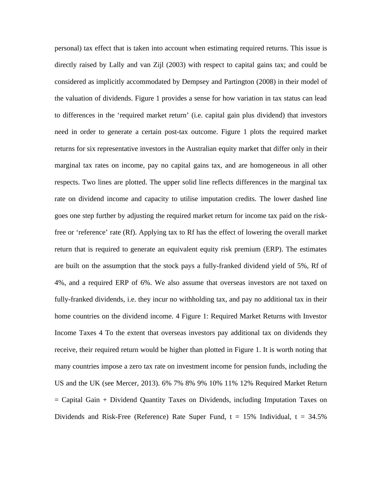
personal) tax effect that is taken into account when estimating required returns. This issue is
directly raised by Lally and van Zijl (2003) with respect to capital gains tax; and could be
considered as implicitly accommodated by Dempsey and Partington (2008) in their model of
the valuation of dividends. Figure 1 provides a sense for how variation in tax status can lead
to differences in the ‘required market return’ (i.e. capital gain plus dividend) that investors
need in order to generate a certain post-tax outcome. Figure 1 plots the required market
returns for six representative investors in the Australian equity market that differ only in their
marginal tax rates on income, pay no capital gains tax, and are homogeneous in all other
respects. Two lines are plotted. The upper solid line reflects differences in the marginal tax
rate on dividend income and capacity to utilise imputation credits. The lower dashed line
goes one step further by adjusting the required market return for income tax paid on the risk-
free or ‘reference’ rate (Rf). Applying tax to Rf has the effect of lowering the overall market
return that is required to generate an equivalent equity risk premium (ERP). The estimates
are built on the assumption that the stock pays a fully-franked dividend yield of 5%, Rf of
4%, and a required ERP of 6%. We also assume that overseas investors are not taxed on
fully-franked dividends, i.e. they incur no withholding tax, and pay no additional tax in their
home countries on the dividend income. 4 Figure 1: Required Market Returns with Investor
Income Taxes 4 To the extent that overseas investors pay additional tax on dividends they
receive, their required return would be higher than plotted in Figure 1. It is worth noting that
many countries impose a zero tax rate on investment income for pension funds, including the
US and the UK (see Mercer, 2013). 6% 7% 8% 9% 10% 11% 12% Required Market Return
= Capital Gain + Dividend Quantity Taxes on Dividends, including Imputation Taxes on
Dividends and Risk-Free (Reference) Rate Super Fund, t = 15% Individual, t = 34.5%

Overseas Investor, t = 10% Interest W/H Tax Resident, t = 0% Individual, t = 47% Key
Assumptions - Investors differ only in marginal tax rates on income, t. They are
homogeneous in terms of their expectations and risk preferences with respect to stocks. -
Fully-franked dividend yield of 5%. Capital gains tax is ignored. - Solid line: Required after-
tax return = Rf + ERP = 4% + 6% = 10% - Dashed line: Required after-tax return = Rf*(1-t)
+ ERP = 4%*(1-t) + 6% Individual, t = 21% Overseas Investor, No Tax Effects Individual, t
= 34.5% Individual, t = 47% www.cifr.edu.au Page 11 There are two messages to take away
from Figure 1. First, there can be meaningful variation in the return that different investors
require a company to deliver as a consequence of tax effects. This is tantamount to saying
that different investors might apply different costs of capital. The issue of how these
differences manifest in the cost of capital that a company should be targeting is discussed in
Section 3.2. Second, it matters what tax effects are included. For instance, our analysis
illustrates how applying tax to the reference asset results in a significant down-shift and
flattening in the overall curve, plus a reordering of the position of various investors on that
curve. Similarly shifts might occur if capital gains tax was incorporated (let alone other
differences across investors). All this hints that tracing tax effects to required returns and
hence cost of capital is far from straightforward. Against this background, a body of literature
addresses the determination of expected returns or cost of capital under the imputation
system. This literature is typically cast within the framework of the Capital Asset Pricing
Model (CAPM), and invokes many simplifying assumptions to make the modeling tractable.
Three approaches are described below, with the main message that the available models vary
in the scope of personal tax effects they incorporate for estimating the cost of capital: •
Officer (1994) models imputation credits as a prepayment of personal income tax, relating it

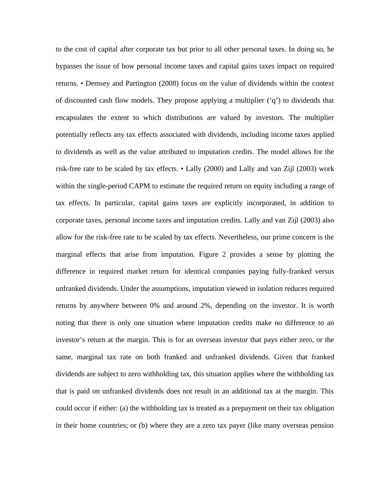
to the cost of capital after corporate tax but prior to all other personal taxes. In doing so, he
bypasses the issue of how personal income taxes and capital gains taxes impact on required
returns. • Demsey and Partington (2008) focus on the value of dividends within the context
of discounted cash flow models. They propose applying a multiplier (‘q’) to dividends that
encapsulates the extent to which distributions are valued by investors. The multiplier
potentially reflects any tax effects associated with dividends, including income taxes applied
to dividends as well as the value attributed to imputation credits. The model allows for the
risk-free rate to be scaled by tax effects. • Lally (2000) and Lally and van Zijl (2003) work
within the single-period CAPM to estimate the required return on equity including a range of
tax effects. In particular, capital gains taxes are explicitly incorporated, in addition to
corporate taxes, personal income taxes and imputation credits. Lally and van Zijl (2003) also
allow for the risk-free rate to be scaled by tax effects. Nevertheless, our prime concern is the
marginal effects that arise from imputation. Figure 2 provides a sense by plotting the
difference in required market return for identical companies paying fully-franked versus
unfranked dividends. Under the assumptions, imputation viewed in isolation reduces required
returns by anywhere between 0% and around 2%, depending on the investor. It is worth
noting that there is only one situation where imputation credits make no difference to an
investor’s return at the margin. This is for an overseas investor that pays either zero, or the
same, marginal tax rate on both franked and unfranked dividends. Given that franked
dividends are subject to zero withholding tax, this situation applies where the withholding tax
that is paid on unfranked dividends does not result in an additional tax at the margin. This
could occur if either: (a) the withholding tax is treated as a prepayment on their tax obligation
in their home countries; or (b) where they are a zero tax payer (like many overseas pension

funds), and can claim a credit for the Australian withholding tax paid. The TDP is effectively
naming overseas investors in this class as the marginal investor. In situations where
withholding tax imposed on unfranked dividends is marginal, then imputation does make a
difference, even for an overseas investor. www.cifr.edu.au Page 12 Figure 2: Difference in
Required Market Return: Fully-Franked less Unfranked Dividends As noted earlier,
imputation may be accounted for in two ways. First is through adding the imputation credit to
the cash flow stream that is made available to investors, prior to considering personal taxes.
Second is as a reduction in the discount rate. Refer to Officer (1994) for analysis and
discussion. Either way, share prices will be higher to the extent that imputation credits are
recognised by the market through either a greater numerator or lower denominator in the net
present value equation. And either way, the return that a company is required to generate
prior to accounting for imputation will be reduced. This amounts to a lowering of the hurdle
rate of return that a company needs to generate on its operations in order to create value –
effectively a reduction in the cost of capital. Another way of seeing this point is that the
operating income that an investment is required to generate is lower to the extent that part of
the corporate taxes paid are remitted as imputation credits, and these credits are valued by
investors as an additional cash flow stream. 3.2. Equilibrium When Tax Status Varies How
tax impacts on share prices and required returns in equilibrium when tax status varies across
investors is far from clear, even in theory. To start with, two approaches to translating
investor demands into equilibrium prices can be found in the finance literature: aggregation
of investor demands, and the ‘marginal investor’ approach. Aggregation of Investor
Demands This approach involves weighting of investor demands, often by the magnitudes
involved and risk aversion. For instance, Brennan (1970) weights tax effects according to the

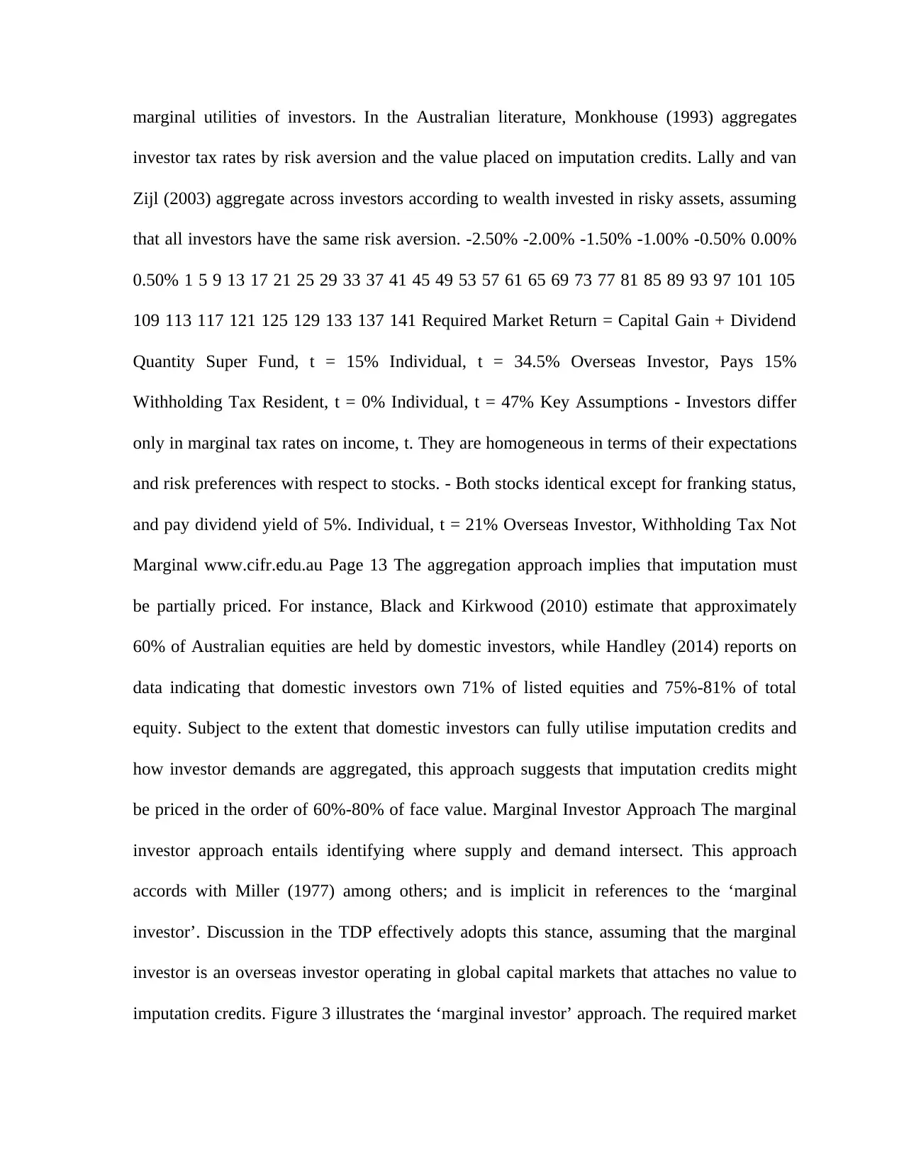
marginal utilities of investors. In the Australian literature, Monkhouse (1993) aggregates
investor tax rates by risk aversion and the value placed on imputation credits. Lally and van
Zijl (2003) aggregate across investors according to wealth invested in risky assets, assuming
that all investors have the same risk aversion. -2.50% -2.00% -1.50% -1.00% -0.50% 0.00%
0.50% 1 5 9 13 17 21 25 29 33 37 41 45 49 53 57 61 65 69 73 77 81 85 89 93 97 101 105
109 113 117 121 125 129 133 137 141 Required Market Return = Capital Gain + Dividend
Quantity Super Fund, t = 15% Individual, t = 34.5% Overseas Investor, Pays 15%
Withholding Tax Resident, t = 0% Individual, t = 47% Key Assumptions - Investors differ
only in marginal tax rates on income, t. They are homogeneous in terms of their expectations
and risk preferences with respect to stocks. - Both stocks identical except for franking status,
and pay dividend yield of 5%. Individual, t = 21% Overseas Investor, Withholding Tax Not
Marginal www.cifr.edu.au Page 13 The aggregation approach implies that imputation must
be partially priced. For instance, Black and Kirkwood (2010) estimate that approximately
60% of Australian equities are held by domestic investors, while Handley (2014) reports on
data indicating that domestic investors own 71% of listed equities and 75%-81% of total
equity. Subject to the extent that domestic investors can fully utilise imputation credits and
how investor demands are aggregated, this approach suggests that imputation credits might
be priced in the order of 60%-80% of face value. Marginal Investor Approach The marginal
investor approach entails identifying where supply and demand intersect. This approach
accords with Miller (1977) among others; and is implicit in references to the ‘marginal
investor’. Discussion in the TDP effectively adopts this stance, assuming that the marginal
investor is an overseas investor operating in global capital markets that attaches no value to
imputation credits. Figure 3 illustrates the ‘marginal investor’ approach. The required market

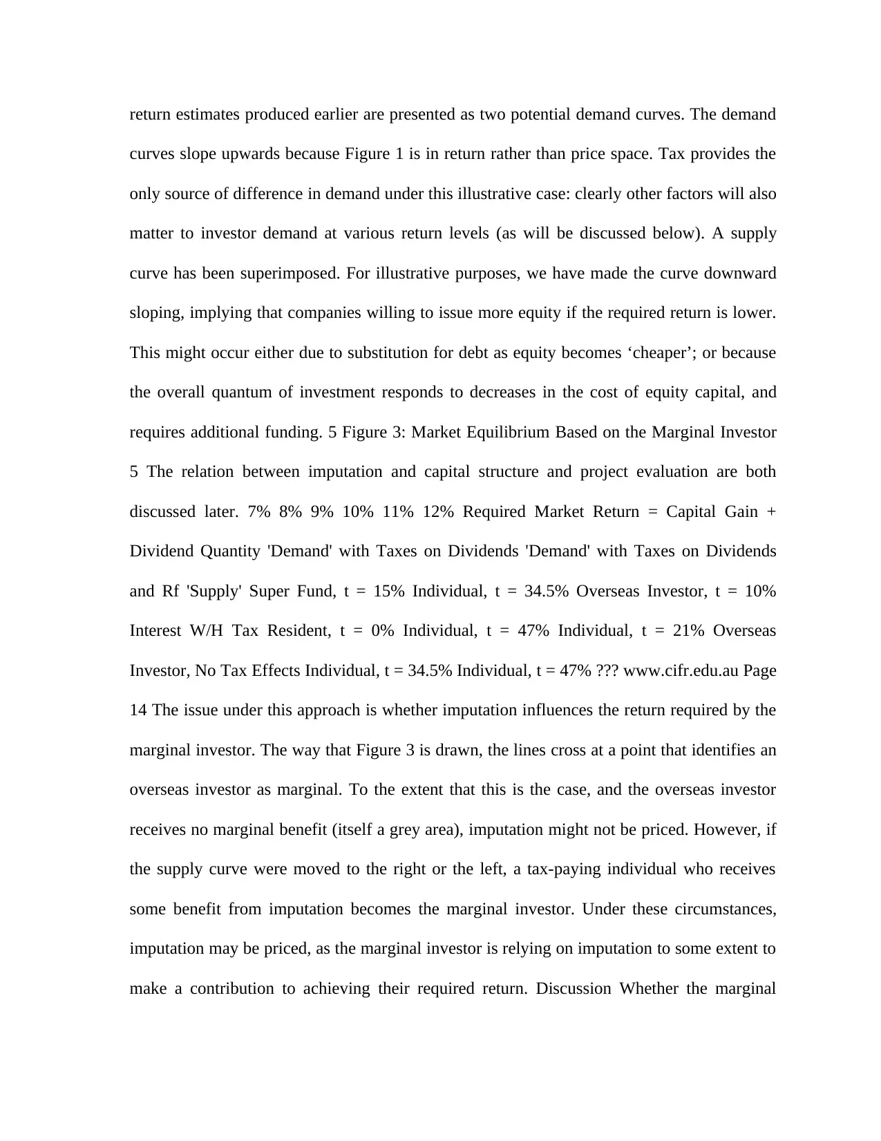
return estimates produced earlier are presented as two potential demand curves. The demand
curves slope upwards because Figure 1 is in return rather than price space. Tax provides the
only source of difference in demand under this illustrative case: clearly other factors will also
matter to investor demand at various return levels (as will be discussed below). A supply
curve has been superimposed. For illustrative purposes, we have made the curve downward
sloping, implying that companies willing to issue more equity if the required return is lower.
This might occur either due to substitution for debt as equity becomes ‘cheaper’; or because
the overall quantum of investment responds to decreases in the cost of equity capital, and
requires additional funding. 5 Figure 3: Market Equilibrium Based on the Marginal Investor
5 The relation between imputation and capital structure and project evaluation are both
discussed later. 7% 8% 9% 10% 11% 12% Required Market Return = Capital Gain +
Dividend Quantity 'Demand' with Taxes on Dividends 'Demand' with Taxes on Dividends
and Rf 'Supply' Super Fund, t = 15% Individual, t = 34.5% Overseas Investor, t = 10%
Interest W/H Tax Resident, t = 0% Individual, t = 47% Individual, t = 21% Overseas
Investor, No Tax Effects Individual, t = 34.5% Individual, t = 47% ??? www.cifr.edu.au Page
14 The issue under this approach is whether imputation influences the return required by the
marginal investor. The way that Figure 3 is drawn, the lines cross at a point that identifies an
overseas investor as marginal. To the extent that this is the case, and the overseas investor
receives no marginal benefit (itself a grey area), imputation might not be priced. However, if
the supply curve were moved to the right or the left, a tax-paying individual who receives
some benefit from imputation becomes the marginal investor. Under these circumstances,
imputation may be priced, as the marginal investor is relying on imputation to some extent to
make a contribution to achieving their required return. Discussion Whether the marginal

investor or aggregation approach better describes how imputation credits become priced in
equilibrium is a point of debate. The marginal investor approach might be seen as more in
keeping with the ‘Economics 101’ notions of price determination, and more consistent with
general equilibrium analysis under which investor demand for (and supply of) imputation
credits is jointly determined with the market clearing price. As a consequence, the marginal
investor approach may assist in analysing the potential effect of changes in the demand
curve. By contrast, aggregating observed demands assumes that investors have found their
equilibrium position given market prices.6 It thus does not directly address how the market
equilibrium emerges in the first place. Nevertheless, the aggregation approach may still
provide a useful description of an existing equilibrium. In any event, the key point is that
there is no clear consensus on the appropriate approach, adding another layer of uncertainty
to the issue of whether imputation credits are priced. An important issue is that both
approaches are often applied as if tax were the only determinant of differences in demand. In
practice, an investor’s demand for assets may reflect a whole range of considerations,
including their expectations, the broader portfolio context, their liabilities, constraints, other
costs, etc.7 This issue is particularly problematic for applying the aggregation approach
through reference to observed holdings, which is the approach typically used in practice. The
fact that a domestic investor holds a stock and can fully utilise any imputation credits does
not provide incontrovertible evidence that they attribute full value to imputation in exchange.
It is entirely possible that a domestic investor could be holding a domestic stock due to
expectations of receiving high pretax returns or other reasons, and not pricing in the
imputation credits in the process. Just because an investor receives imputation credits does
not necessarily mean they fully price them, and hence require a commensurately lower pre-

imputation return from the company as a consequence. The existence of influences other than
tax is also problematic for the marginal investor approach. Tax considerations may be only
one of a raft of factors that are determining pricing at the margin. This makes identifying the
marginal investor much more complex than merely assuming it must be the investor who gets
least value out of imputation, i.e. overseas investors. The marginal investor could be one for
whom imputation credits form part of the overall ‘package’ of effects that entice them to hold
a stock. 8 For instance, the marginal investor might be a domestic investor who is relatively
pessimistic on the company’s outlook, and imputation matters because it gets them over the
line. Meanwhile, it is not impossible that overseas investors might sit lower down on the
demand curve, say because they are keen buyers for some other reason, such as optimistic
expectations. In these situations, imputation credits could get priced to some extent as part of
enticing the last investor in at the margin. Essentially we are saying that drawing demand
curves reflecting only tax differences is too simplistic. 6 Monkhouse (1993) explicitly states
this assumption. 7 This focus on tax alone is encouraged by the manner in which tax effects
are modeled. The models are mostly partial equilibrium models where all other factors are
assumed constant. The world does not work this way. 8 Imputation may similarly be one of a
range of factors that influences trading patterns, most notable around exdividend dates (see
discussion in Section 4.2). www.cifr.edu.au Page 15 Another issue is that the identity of the
marginal investor may be a moving feast, varying across stocks or time. Hence the pricing of
imputation credits could be conditional, rather than a universal constant. Some stocks may be
held entirely by local investors who value imputation credits, and thus become priced for
lower expected market returns. One potential area is the small cap sector, where interest from
overseas investors is typically low (which will be discussed in Section 8.1). Meanwhile other

stocks may need to attract those who are unable to utilise imputation credits, like overseas
investors, in order for the market to clear. The possibility of segmented pricing is consistent
with the findings of Durand, Limkriangkrai and Smith (2006) with regard to large versus
small Australian stocks. It is also consistent with the findings of Jun and Partington (2014)
that dividends on ADRs are priced as though they are traded by US investors, while
dividends on the underlying stocks are priced as though they are traded by Australian
investors who value the imputation credits. The identity of the marginal investor may change
over time in reflection of whoever is active in the market. The availability of imputation
credits (or otherwise) might attract a particular clientele in certain situations. For example,
Chu and Partington (2008) find that the pricing of parallel CRA bonus issues with differing
entitlements to imputation credits varied with proximity to the dividend payment. These
authors interpret this finding as consistent with dividend values being set by short-term
traders around the ex-dividend date, and by long-term investors at other times (although they
also find substantial value is attached to the franking credit at all times). A related issue is
how the pricing of dividend events might accord with the determination of price levels and
returns over longer holding periods. One possibility is that the pricing around dividend events
may be set by investors who trade to limit the incidence of tax, or capture imputation credits.
Ainsworth et al. (2010, 2015) examine institutional trading and share prices around ex-
dividend dates, and find evidence consistent with tax motivations as an explanation for the
observed patterns. Meanwhile, the overall price level and hence longer-term (say year-to-
year) expected returns could be dictated by another class of investor who might only become
active in response to substantial shifts in prices or long-term expected returns. We will return
to this issue in Section 4, as it is relevant for interpreting drop-off and comparative pricing

studies relative to those examining prices and returns. The discussion is this section raises
more issues than it offers resolutions. But this is the key point. The manner in which
imputation is priced by the market is quite unclear in theory. It is also going to be inherently
difficult to extract in practice, given that imputation is just one of many effects that determine
share prices, and the limited scope for clean experiments. 9 The fact that the value attributed
to imputation credits might also vary across stocks and through time only compounds the
problem. 3.3. What Tax Effects Are Taken Into Account? There is no question that
imputation and other tax effects affect the net returns actually achieved by investors.
However, just because investors incur taxes does not make it a foregone conclusion that
those taxes are taken into account when making investment. Imputation is just one of many
considerations, and need not be germane to the investment decision. The manner in which
imputation and other tax effects are incorporated may be affected by the fact that investment
decisions are often made under agency arrangements, and by various behavioural effects. At
this point we merely flag the issues, in order to provide background for later discussions of
actual practice. 9 Some clean experiments have been done, such as Walker and Partington
(1999) and Chu and Partington (2008). However, such experiments only examine the pricing
of dividends and any attached imputation credits (i.e. they do not examine whether
imputation is capitalised into the overall price level). They also exploit special situations that
may not apply to all stocks. Consequently, while the valuation of distributed imputation
credits has high validity under these studies, their generalisability is open to question.
www.cifr.edu.au Page 16 The first issue is whether investors take imputation into account
when pricing stocks and/or setting their portfolios. There are reasons why this may not
necessarily be the case, even where imputation is of value. Much investment occurs under

delegated management, i.e. it is undertaken by fund managers, rather than the beneficial
investor. The question arises as to whether fund managers allow for tax effects, given their
incentive structures and the often opaque tax status of their end-investors. Behavioural issues
may arise, such as whether tax is salient, or the extent to which decisions are based on
something other than rigorous analysis. Tax might also be ignored because it is considered a
second-order effect, relative to aspects like the potential operating outlook for a company.
The second issue is whether companies allow for imputation in determining their cost of
capital, and making decisions. The fact that companies are managed under agency
arrangements raises questions over whether management has reasons or incentives to
consider imputation. When contemplating the corporate perspective, it is useful to distinguish
tax effects that are incurred by the company directly, versus those that are incurred by its
shareholders. Company tax is the main tax effect that is directly incurred by the company. As
company tax impacts on earnings, it is highly likely to be of concern for management. For
other taxes incurred by the shareholder – those related to dividends, imputation credits and
capital gains – it is not immediately apparent that they will be considered by management.
Incentive structures and opacity around the tax status of shareholders may dull the motivation
to take these effects into account. Nevertheless, one distinguishing feature of imputation is
that companies have some control over the amount of credits they earn and distribute.
Meanwhile, management is aware that imputation credits are of value to many shareholders.
This increases the chances that imputation may be taken into account, relative to (say) capital
gains taxes. Observing behaviour is one way of ascertaining how tax effects are actually
taken into account. A theme running through this report is that more attention should be paid
to how imputation impacts on behaviour, rather than just focusing on how it affects the

computations like cost of capital estimates. In the sections that follow, we try to convey what
is known about the link between imputation, other tax effects, and behaviours.
7. Review of issues raised by Frontier Economics in connection with Ausgrid’s 2019-24
regulatory
1. Introduction Ausgrid has made a revenue proposal to the Australian Energy Regulator
(AER) in connection with its 2019- 24 regulatory period. Its proposal includes a report that
Ausgrid commissioned from Frontier Economics (2018) entitled Estimation of certain aspects of
the regulated rate of return. The Frontier report was prepared by Dr Stephen Gray, who is
Professor of Finance at the University of Queensland Business School. Energy Consumers
Australia has commissioned the South Australian Centre for Economic Studies (SACES) to
prepare a very short expert report on matters raised in the Frontier study. This SACES report has
been prepared by Mr Jim Hancock, Deputy Director. Many of the issues raised by Frontier have
recently been discussed during the AER’s consultations over the preparation of its 2018 Rate of
Return Guideline. As part of those consultations the AER held two expert evidence sessions in
March and April 2018. In the first session, experts discussed discussion papers relating to
gearing, financial performance measures, and risk and judgement. In the second session experts
discussed gamma, equity beta, and MRP (market risk premium), risk free rate averaging period
and automatic application. The agenda of the second session—which the author Jim Hancock
attended as an expert—is closely related to the matters covered by Frontier. Then, in July 2018,
the AER released Draft Guidelines. The Draft Guidelines address key issues arising in Frontier.
Among other things, they propose:  a risk free rate based on an average of synthetic 10-year
Commonwealth bond rates;  an equity beta of 0.6;  a market risk premium of 6 per cent; and 
a gamma of 0.5. It is possible that some of the matters presently under consideration by the AER

in the Ausgrid decision will be resolved by a proposed “binding rate of return instrument”. The
instrument has been proposed by the COAG Energy Council and draft legislation to give effect
to it has been published but has not at this stage been enacted. However, as the instrument has
not been brought into force, and may not be, this submission addresses Frontier’s work on the
Ausgrid proposal under the assumption that no binding instrument is in place. This review of
Frontier proceeds in line with the chapter structure used by Frontier. It draws on the discussions
in the second expert evidence session and in particular on the Expert Joint Report that was
prepared by Cambridge Economic Policy Associates (2018) and also on the recent Draft
Guidelines (AER 2018a). Page 2 Review of issues raised by Frontier Economics July 2018 South
Australian Centre for Economic Studies, University of Adelaide 2. Equity beta Frontier’s main
conclusions are:  Frontier says that in a series of decisions, the AER has explained that: (a) It
considers the “best empirical estimate” of beta to be 0.5; and (b) The allowed beta is to be set to
0.7 due to three additional considerations: (i) “international estimates” – the fact that the weight
of evidence from international comparators supports a beta estimate materially above the AER’s
domestic starting point estimate of 0.5; (ii) “consideration of the theory of the Black CAPM” –
the fact that the Black CAPM evidence is that the unadjusted SL-CAPM will systematically
understate the required return on low-beta stocks; and (iii)“investor certainty” – the fact that
instability in equity beta allowances may cause investors to increase their assessment of
regulatory risk.” [pp. 4-5]  Frontier says that on the available evidence the “best empirical
estimate” of beta has increased to 0.7.  Beta estimates for regulated network comparators that
have delisted are increasingly out of date and they cannot pick up on movements in beta since
delisting.  Beta estimates have increased since the 2013 Guideline for the listed regulated
energy network comparators and for other relevant comparators.  Continued application of the

2013 Guideline approach with allowance for the latest “best empirical evidence” supports a beta
of at least 0.7. SACES Response: 1. AER (2017) explicitly rejects Frontier’s characterisation of
its decision process on beta. It says “Frontier has mischaracterised our approach for equity beta.
We do not uplift the equity beta to 0.7 (from 0.5) to account for the low beta bias. We select a
top of the range value of 0.7 (from a range of 0.4–0.7) to account for the theory of the Black
CAPM and other relevant information.” [pp. 3-67] It goes on to say that it uses a 2014 report by
Professor Olan Henry to inform its beta decision and that “we give most consideration to
empirical Australian estimates of suitable comparator firms (Australian energy network firms)
which indicate a range of 0.4–0.7 … Our consideration of the theory of the Black CAPM and
international estimates (which we give less consideration) suggest a point estimate towards the
upper range. These considerations along with our consideration of investor certainty lead us to
set a point estimate of 0.7.” [p. 3-165] 2. The 2013 Guideline adopted a value of 0.7 for beta,
which was at the top end of its identified range. 3. When it chose the beta value of 0.7, the AER
was mindful that its existing practice was to use a value of 0.8, and it was concerned that it
should not make too large adjustments to the beta parameter. It wanted to adjust parameters
gradually so as to minimise perceptions of regulatory risk. With the passage of 5 years since the
2013 Guideline, it is consistent with that gradualist approach for the AER to now adjust beta
lower if it believes that the best estimate is lower than 0.7. 4. Since the Henry (2014) report was
prepared there has been a reduction in the number of listed Australian energy networks and this
complicates the task of estimating contemporary betas for energy networks. The number of listed
Australian regulated networks has fallen from 9 at the time of the Henry study to 4 at the time of
the last AER analysis and to 3 today. The AER could base its beta estimates on the remaining 3
listed entities but this is a fairly thin dataset. 5. Frontier analyses betas for the 4 entities that were

listed at May 2017. It finds that the central point estimates of beta for a portfolio of these entities
have risen. However, it does not address whether the changes are statistically significant. 6.
There are two primary approaches to augmenting the beta observations available to AER. First,
one could come up with new comparators and directly impute the regulatory beta from the
observed betas on the new comparators. Secondly, one could combine the historical beta
estimates for regulated energy networks with an estimate of change in beta based on a set of
comparators that has the necessary data to carry out a matched sample comparison of betas at
different points in time. 7. An example of the first approach is the proposal by Frontier to
consider betas for a set of transportrelated Australian infrastructure firms that Frontier says have
common characteristics to the Australian regulated energy networks. Frontier finds that these
entities have betas which are materially higher than the AER’s current beta of 0.7 and argues that
“if this evidence were to be afforded any weight, the result would be an increase in the equity
beta allowance” [p. 27]. In our view, the fact that these beta estimates Review of issues raised by
Frontier Economics Page 3 South Australian Centre for Economic Studies, University of
Adelaide July 2018 for the transport sector are higher primarily suggests that they may not be a
very good comparators for the regulated energy networks. 8. A second example of finding new
comparators is the suggestion made from time to time that the AER should use betas estimated
overseas for comparable firms. It seems to us that this approach is fraught with problems. One
problem is that the nomination of a relevant comparator group is highly judgmental. The
discussion of evidence from international comparators in AER (2013b) shows that there is a
quite wide range of levels for the beta estimate depending on: which firms are regarded as
comparators; what time period is used to observe the comparators; and the method used to
aggregate comparators. Even if one focuses on regulated energy networks, there are remaining

questions about the comparability of the regulatory frameworks and approaches to their
application, differences in the surrounding institutional frameworks, exposures to worker pension
liabilities and assets held against them, etc. A second problem is that beta estimates also depend
on the market portfolio that is used as a benchmark for covariance calculations. If, as is widely
believed to be the case, the Australian market on average is rather more volatile than
international markets as a result of compositional factors such as Australia’s exposure to
resource industries, then betas for Australian regulated networks on the Australian market might
quite plausibly be lower than the betas calculated for, say, US regulated networks on the US
market. 9. The alternative of tracking changes in beta is also problematic, in this case because the
data tend not to provide much strong evidence of sustained changes in betas. Analyses appear to
be quite vulnerable to shifting the start and end points of the data series used in analysis. AER
(2018b) presents average annual betas for the Australian utilities sector which show an average
beta of 0.63 for the 5 years to 2017 compared with 0.5 for the 5 years to 2012. But the difference
appears not to be statistically robust. The point is illustrated by noting that, notwithstanding the
higher average of the past 5 years, as recently as 2016 the recorded beta for the utilities sector
was 0.4. 10. It is clear from the estimates that betas fluctuate over time. But this does not mean
that the latest observation tells us very much about what betas to expect in the coming few years.
Unless one can establish evidence of random walks or trends in the data then we should not put
too much weight on the latest observation; rather we should regard it as one more piece of
evidence to assist with estimating the noisy random variable beta. 11. In its Draft Guidelines the
AER says that the empirical evidence “supports an empirical range of 0.4–0.8 with clustering in
the 0.5–0.6 range. We consider our comparator set of domestic firms is the best empirical guide
currently available” [p. 243]. The AER also says that one factor behind its decision to hold beta

at 0.7 in the 2013 Guidelines was that while a more substantial downward adjustment was
probably warranted on the data by itself, a more gradual approach to adjustments was desirable
in the interests of investor certainty. The AER says that it is consistent with that gradualist
approach to now move beta lower if the evidence warrants it. 12. Our conclusion is that
Frontier’s call to increase the beta estimate from the AER’s existing norm of 0.7 is not
convincing. If beta were revised downward modestly from 0.7 this would take it closer to the
middle of the range of beta estimates that have been made over the years while maintaining a
gradualist approach to adjustment. Page 4 Review of issues raised by Frontier Economics July
2018 South Australian Centre for Economic Studies, University of Adelaide 3. Low-beta bias
Frontier’s main conclusions are:  The phenomenon of low-beta bias is a standard phenomenon
that is covered in textbooks.  The majority of studies support an estimate of the zero-beta
premium between 2% and 4%. This is slightly above the range of 1.5% to 3% that was
nominated by the AER as “reasonable” and “open to us” in its 2013 Guideline.  The AER says
that it allows for low-beta bias by making an upward adjustment to the equity beta in the SL-
CAPM. The adjustment that the AER makes is consistent with zero-beta premium of at most
2.6% and Frontier concludes that the AER’s approach “does not appear to fully correct for low-
beta bias. A full correction for the observed low-beta bias would require a greater uplift to the
statistical beta estimate than that which the AER has adopted in recent decisions” [p. 39].
SACES Response: 1. Much of the evidence that Frontier presents in support of low-beta bias
relates to the US. 2. Although the two Australian empirical studies1 are suggestive that the zero-
risk premium is greater than zero, they certainly are not conclusive. There are questions as to the
robustness of statistical tests used in the studies. And ignoring those questions, the estimates
taken at face value have such wide error margins that conventional 95 per cent confidence testing

would seem to admit any estimate within plus or minus 10 percentage points of the authors’
central estimates. See Box 1 for further discussion. 3. Professor Kevin Davis’ (2011) expert
advice to the AER regarding the Black Scholes model and its implications for Australian
regulatory decisions remains relevant. Davis notes inter alia that:  there is a theoretical basis for
SL-CAPM and one should be wary of preferring atheoretic specifications on the basis of
empirical studies which have ambiguous interpretations;  tests of the SL-CAPM rely on an
assumption of market efficiency, and when the test is rejected it is possible that mean-variance
efficiency rather than SL-CAPM is what is rejected;  neither beta’s nor expected returns on
stocks are actually observed and they are instead proxied with historic realisations, which may
go some way to explaining the poor empirical performance of SL-CAPM ;  restrictions on
financing that are allowed for in the Black CAPM do not seem large enough to justify the
magnitudes of estimates of the zero-risk premium; and  test statistics that are relied on in many
studies are not valid, leading to unwarranted rejections of SL-CAPM. In our view these
arguments remain valid today. 4. In conclusion, we are not convinced of Frontier’s claim that the
AER makes inadequate adjustment for low-beta bias. In fact it is possible that the current
allowance goes too far. There is no convincing argument to increase the existing allowance for
low-beta bias. Box 1:Estimates of the zero-beta premium in Australia NERA (2013) present a
number of alternative estimates of the zero-beta premium using Australian data. Their central
point estimates are extraordinarily high—e.g. for the case of a portfolio using data from 1974 to
2012 they estimate a 13.95 per cent zero-beta premium which would mean that a zero-beta
portfolio could be expected to earn 14 per cent in excess of the bond rate. The standard errors on
their estimates are also very high at 5.48 per cent and, using a rough rule of thumb, they suggest
a confidence interval of plus or minus 11 per cent around that central estimate. On the basis of

this NERA conclude that the hypothesis “zero-risk premium equals market risk premium” would
not be rejected for any of the commonly discussed values of the MRP. And they conclude that
the hypotheses of “zero premium over the bond rate” is rejected. However, in my view it is
questionable whether very much can be taken from the NERA results, as they are very imprecise.
That concern is reinforced when one takes into account that the estimation of standard errors in a
setting like this is not straightforward and the risk is that the standard errors are even larger than
estimated. For example, the authors give no indication that they have adjusted their results to
make them robust against heteroscedasticity yet this is likely to be a problem in the modelling of
security prices. In conclusion, probably the most that can be drawn from NERA’s results is that
they suggest that the zero-beta premium in Australia is non-zero, but with the use of a model that
is imprecise and at risk of misspecification. SFG estimate the zero-beta premium in a model that
seeks to control for the influence of book-to-market ratios (BMRs). They do this by selecting
stocks to portfolios on the basis of industry, size and BMR. SFG report that on their most basic
specification “The zero-beta premium … is 3.34% per year”. Yet this is only a central point
estimate and using the 1 NERA (2013) and SFG Consulting (2014). Review of issues raised by
Frontier Economics Page 5 South Australian Centre for Economic Studies, University of
Adelaide July 2018 standard errors published by SFG shows that the conventional 95 per cent
confidence interval ranges includes zero. (SFG report a 90 per cent confidence interval, and by
this device have a confidence interval that does not include zero.) And none of the other
specifications that the authors consider give a more convincing case for a zero-beta premium in
excess of zero. There are also unexplained aspects of SFG’s analysis, such as how standard
errors have been adjusted to allow for the overlapping data structure that SFG employed,
robustness to heteroskedastic data generating processes, etc. In conclusion, this study covers

essentially the same data as NERA and does not produce any more compelling evidence in
favour of a substantial zero-beta premium. Page 6 Review of issues raised by Frontier
Economics July 2018 South Australian Centre for Economic Studies, University of Adelaide 4.
Market Risk Premium Frontier’s view:  The historical excess returns data—considered over 5
averaging periods with a varying amount of history—support an MRP in the range 6.0% to 6.5%.
 Frontier argue that the total required rate of return on equity has not fallen along with real
interest rates in recent years.  Application of the Dividend Growth Model (DGM) suggest an
MRP range of 7.14% to 8.18%.  The preponderance of evidence indicates that the MRP has
increased since the AER’s Guideline.  Market evidence indicates that a reasonable estimate of
the MRP is at least 7%. SACES response: 1. It is quite consistent with the theoretical
underpinnings of the MRP that it may vary through time. For instance, theoretical considerations
imply that changes in perceptions about the riskiness of the market should cause the MRP to
change. 2. Models to estimate the MRP suffer from high variances—i.e. imprecision—and the
best way to deal with this is to have more observations. This means that it is desirable to have a
long series of returns to estimate the MRP. While structural models that estimate a time-varying
MRP—possibly contingent on other variables—are reasonable in principle there has not been
much success finding time-varying models that convincingly outperform simple averages of
historical data. We acknowledge that it will at times be appropriate to make adjustments to raw
data when there are strong in-principle arguments for it, even if those arguments are not
statistically testable. An example is adjusting historical excess returns from 1988 onward to
allow for the value of franking credits distributed. 3. Historical averages of 1-year excess returns
over the bond rate—inclusive of the value of franking credits—are in the range 6.0% to 6.5%. 4.
An important issue which has not yet received the attention it deserves is that the emphasis on 1-

year return horizons leads to higher MRP estimates than when a longer horizon is considered.
Average annual returns calculated from a sample of multi-year intervals are lower than the
average annual returns calculated on a sample of 1-year intervals—see Appendix A. There
should be no presumption in favour of a 1-year horizon. The CAPM says nothing about the
horizon that should be modelled. The use of an average of 1-year returns is simply a default
outcome that reflects common practice and an implicit assumption that the return duration does
not matter. But multiyear durations are more relevant than 1-year durations for network
regulation and efficient network investment signals because network investments have lives of
many years. The building blocks calculation of return on equity actually uses a 10-year risk free
rate, and while this is not determinative of the analysis horizon it does tend to confirm that a
lengthy investment horizon is relevant for network investment decisions. Taking these concerns
into account, the historical data suggest an MRP—inclusive of the value of franking credits—in
the range 5% to 6%. 5. The question of what length of analysis horizon to use also touches on the
debate about whether to use arithmetic or geometric averages of data. In general an arithmetic
average of 1- year returns will be a better estimator of a 1-year return than a geometric average
over a multi-year period. But a compound of the arithmetic average of 1-year returns will not be
a good estimate of the expected return on an investment with a life of several years and it will in
fact tend to exaggerate the expected return. Although the arithmetic average of 1-year returns has
good credentials as an estimator of average 1-year returns, this does not mean that it has good
credentials as an estimator of required returns for long-lived assets. 6. Frontier’s claim that the
required rate of return on equity has not fallen one-for-one with bond rates is equivalent to
saying that the MRP has risen in recent years. Neither the CAPM nor mainstream theories of the
consumer and the firm provide any rationale for a negative correlation between MRP and bond

rates. But we acknowledge that this still leaves open the possibility that a correlation exists. If a
correlation between MRP and bond rates exists, then a correlation between historic excess
returns and bond rates should exist too. We regressed excess returns on bond rates using the
AER’s long series of annual excess returns which has 135 annual observations. We find no
evidence of a statistically Review of issues raised by Frontier Economics Page 7 South
Australian Centre for Economic Studies, University of Adelaide July 2018 significant
relationship—Appendix B. However, we acknowledge that the data lead to a test with very weak
power. If the data do not reject the competing hypothesis that the MRP moves inversely one-
forone with bond rates. Frontier points to estimates of the required rates of return on equity in
support of its argument that they have not fallen in line with bond rates. But they are only
estimates and these estimates are constructed using DGM models which at any point in time
typically assume that required rates of return on capital are constant into the future (see Lally
2013). That very assumption is likely to impart stability to the series of total return estimates.
The apparent stability of required rates of return in the face of fluctuations in bond rates may in
fact be an artifice of the method used to estimate required total rate of return. 7. The fact that
Frontier’s DGM-based range for the MRP is so much higher than the range based on historical
excess returns invites the question as to why the divergence arises. We do not have the data to
carry out the reconciliation, but the likely answers relate to the structure of DGM estimates and
to the parameter assumptions used by Frontier. When the DGM is applied conventionally, it
solves for a stable-through-time cost of equity. An MRP estimate that is calculated residually by
deducting a bond rate will then fluctuate inversely to the estimated required rate of return on
equity. As was argued in the previous point, there is neither theory nor empirical evidence to
support the assumption that MRP does fluctuate inversely with the bond rate. On the matter of

parameter assumptions, we note that Frontier’s central DGM scenario employs a 4.6 per cent
growth assumption which is consistent with the 4.6 per cent scenario put forward in Lally
(2013). Lally’s assumption was based on 3.0 per cent real GDP growth, 2.0 per cent real growth
in dividends per share and 2.5 per cent CPI. While a 3.0 per cent GDP growth rate is probably
reasonable for today’s outlook, dividend payout ratios in Australia have been high over the last
decade—notwithstanding with some apparent reduction over the last two years or so—and this
has potentially undermined prospective growth rates for dividends per share. In our view
Frontier’s DGM estimates of required return on equity—indeed any DGM results—should be
viewed as highly judgmental. DGBM estimates have the potential for significant departures—
upside and downside—from the true but unobservable required returns on equity. Moreover, they
carry an implicit assumption that MRPs move up when bond rates fall (and move down when
bond rates rise) but this supposition is supported neither by theory nor by the empirical
evidence.. 8. In conclusion, we believe that the AER should take account of the fact that its
regulatory rate of return is intended to guide long-lived investment decisions and that estimates
of annual returns based on long durations are appropriate. Estimates based on historical averages
are more appropriate than estimates based on DGM. It is appropriate to adjust the historical
average data where there are strong a priori grounds for doing so and on this basis the MRP
estimate should—as is the case in the AER calculations—take into account the value of franking
credits distributed. In view of these factors an MRP in the middle of the range 5% to 6½% is
warranted. The MRP of 6 per cent that the AER proposes in its Draft Guideline seems reasonable
although perhaps conservative towards the high side. Page 8 Review of issues raised by Frontier
Economics July 2018 South Australian Centre for Economic Studies, University of Adelaide 5.
Gamma Frontier’s view:  There is broad agreement that 𝛾 should be interpreted as the product

of a distribution rate 𝐹 and a second parameter 𝜃, i.e. 𝛾 = 𝐹 × 𝜃.  Frontier believes that 𝜃
should be set equal to the “value of distributed imputation credits” and opposes the existing AER
approach which is to equate 𝜃 with the “utilisation rate”.  Frontier says that the AER’s use of
the “redemption” or “utilisation” approach to calculating gamma results in “an internally
inconsistent implementation of the regulatory model whereby investors are properly
compensated for all personal taxes and costs that apply to dividends and capital gains, but not
compensated at all for the additional personal costs that apply to imputation credits” [p. 169]. 
Frontier says that if a calculation gamma is made using the redemption approach then
acknowledged deficiencies with the ATO data are not a problem because the errors cancel out in
the calculation. The ATO data support a redemption-based gamma estimate of 0.34. SACES
response: 1. The role of 𝜃 is to make an estimate of 𝛾 using the formula 𝛾 = 𝐹 × 𝜃. The
estimate of 𝛾 is used to adjust the corporate tax element in the building blocks calculation of cost
of capital. The corporation tax payments by the entity—which are made at the statutory tax rate 𝑡
—are discounted to allow for subsequent refunds against franking credits. The amount that is
refunded depends on the distribution rate and the utilisation rate. This interpretation is made
clear in, for instance, clause 6.5.3 of the National Electricity Rules (v. 111) which says “The
estimated cost of corporate income tax of a Distribution Network Service Provider for each
regulatory year (𝐸𝑇𝐶𝑡 ) must be estimated in accordance with the following formula: 𝐸𝑇𝐶𝑡
= (𝐸𝑇𝐼𝑡 × 𝑟𝑡) (1 – 𝛾) where: 𝐸𝑇𝐼𝑡 is an estimate of the taxable income for that regulatory
year that would be earned by a benchmark efficient entity as a result of the provision of standard
control services if such an entity, rather than the Distribution Network Service Provider, operated
the business of the Distribution Network Service Provider, such estimate being determined in
accordance with the post-tax revenue model; 𝑟𝑡 is the expected statutory income tax rate for that

regulatory year as determined by the AER; and 𝛾 is the value of imputation credits.” [p. 765] In
our view it is entirely consistent with the Rule to identify 𝜃 as a utilisation rate and this is the
view of the Federal Court. If 𝜃 is set at the utilisation rate then 𝐸𝑇𝐶𝑡 represents the
corporation tax paid to the ATO net of the credits granted against it. 2. The return on an equity
comprises three benefit streams: capital gains on the disposal of an equity, dividends paid and
imputation credits distributed. An investor may value a dollar delivered through these income
streams differently, for instance as a result of different tax treatments (e.g., for an Australian
resident capital gains are likely to be taxed at lower rate than dividends), transaction costs and
administration costs. One empirical investigation of these issues is Frontier (2016) and the results
of their Model 4 indicate that $1 of dividend is on average valued at $0.91 of capital gain and $1
of distributed imputation credits is valued at $0.36 (which on the basis of a utilisation rate of 0.6
would imply a value of 60 cents in the dollar for utilised imputation credits). 3. Frontier’s
assertion that there is an inconsistency in the treatment of, on the one hand, dividends and capital
gains and, on the other hand, franking credits, is misleading. It is possible that capital gains and
dividends have different “market values”—and as noted in the previous point Frontier has
previously claimed that they do have different market values—yet the AER makes no allowance
for this. In particular, the historical excess returns data that are calculated by AER and used as
the primary basis for determining MRP comprise dividends valued at $1 in the dollar, capital
gains valued at $1 in the dollar, and imputation credits valued at 60 cents in the dollar (based on
60 per cent utilisation). A similar issue arises with respect to the DGM: the DGM estimate of the
cost of capital is calculated purely with reference to dividends exiting the entity and without
regard for the different valuations that investors may place on dividend and capital gain benefits.
4. The AER’s existing treatment is by implication one in which benefit streams to stockholders

from an entity are valued ex the entity and gross in the hands of the stockholder. The various
costs that are incurred by the stockholder in realising and administering those gross benefit
streams undoubtedly impact on the net benefits accruing to the stockholder but because the AER
is not focussing on the net Review of issues raised by Frontier Economics Page 9 South
Australian Centre for Economic Studies, University of Adelaide July 2018 benefit streams it
does not use market valuation data to mark down the gross benefits. It is consistent with this
view that 𝜃 be regarded as a pure utilisation rate. 5. In our view it seems desirable that there be a
consistency between the way that benefit streams—capital gains, dividends and franking credits
—are aggregated to estimate the MRP and the parameter values that are adopted elsewhere in the
WACC. 6. It is acknowledged, including by Frontier we think, that there are substantial quality
problems with the ATO data on franking credit distributions. We agree with Frontier that so long
as one has good data on franking credits created and franking credits claimed, this should not
matter if the objective is to estimate gamma for the universe of entities in the ATO tax collection.
This is so because the estimate of franking credits distributed then cancels out in the calculation
of gamma. With this in mind Frontier says that the ATO data support a redemption-based gamma
estimate of 0.34. 7. Frontier expresses confidence that the ATO franking credits created and
franking credits claimed data are of good quality and also implies that they are well suited to the
calculation of gamma. We are unsure about the quality of the ATO data for these items. While
we are sympathetic to Frontier’s view that the ATO should have reliable data we would say the
same for franking credits distributions, and the deficiencies in the distribution data bring into
question the quality of the other data. The fact that the ATO seemingly should have good data
does not convince us that it actually does have good data. 8. There is also a question as to
whether the entities in the ATO collection are a suitable benchmark for estimating gamma.

Given the emphasis on estimating WACC parameters from observable data for listed companies,
there is a case for seeking to confine gamma to listed companies. There is also a case for
confining the estimate to large companies and perhaps also to companies in the same industry
sector as the regulated network entities. 9. We note that in its recent Draft Guidelines for rate of
return the AER (2018a) has taken a distribution rate of 0.83 and a utilisation rate of 0.6 and
arrived at a gamma value of 0.5. The distribution rate assumption takes into account: Professor
Lally’s finding of a distribution rate of 0.88 from the financial reports of the top 20 ASX listed
firms; a distribution rate of 1 for comparators from the same industry as the BEE [p. 397]; and
ATO data suggesting distribution rates, over all equity, of either 0.76 (FAB basis) or 0.57
(dividend data basis). The AER says that its assumed utilisation rate is slightly lower than is
suggested by ABS data on equity ownership (foreign versus domestic owner shares). 10. On the
basis of these considerations, we feel that the AER should use a utilisation-based estimate of 𝜃
and should use distribution rate data observed from appropriate ASX-listed comparator firms.
The gamma estimate of 0.5 in the Draft Guidelines is reasonable in light of these considerations.
Page 10 Review of issues raised by Frontier Economics July 2018 South Australian Centre for
Economic Studies, University of Adelaide References Australian Energy Regulator (2013a),
Better Regulation. Rate of Return guideline. December. https://www.aer.gov.au/ Australian
Energy Regulator (2013b), Better Regulation. Explanatory Statement. Rate of Return guideline.
December. https://www.aer.gov.au/ Australian Energy Regulator (2017), Draft Decision.
TransGrid transmission determination 2018 to 2023. Attachment 3 – Rate of return. September.
https://www.aer.gov.au/ Australian Energy Regulator (2018a), Draft. Rate of return guidelines.
Explanatory Statement. July 2018. Australian Energy Regulator (2018b), Discussion Paper.
Equity beta. Ausgrid (2018), Ausgrid’s regulatory proposal.1 July 2019 to 30 June 2024.

https://www.aer.gov.au/ [Accessed 20 June 2018] Cambridge Economic Policy Associates
(2018), Rate of return guideline review – facilitation of concurrent expert evidence. Expert Joint
Report. April. https://www.aer.gov.au/ Davis, Kevin (2011), Cost of Equity Issues: A Report for
the AER. January 16. Frontier Economics (2018), Estimation of certain aspects of the allowed
rate of return. A report prepared for Ausgrid. April. https://www.aer.gov.au/ Grundy, Bruce
(2010), The calculation of the cost of capital: A report for Envestra. September 30. Henry, Ólan
T. (2014), Estimating β: An update. April. Lally, Martin (2013), Review of the AER’S proposed
dividend growth model. December 16. NERA Economic Consulting (2013), Estimates of the
Zero-Beta Premium. A report for the Energy Networks Association. June. SFG Consulting
(2014), Cost of equity in the Black Capital Asset Pricing Model. Report for Jemena Gas
Networks, ActewAGL, Networks NSW, Transend, Ergon and SA Power Networks. May 2014.
8. Understanding the economy wide efficiency
1. INTRODUCTION The main taxes used in Australia to raise government revenue lead to
losses in economic efficiency by distorting price signals and thereby changing the behaviours of
individuals, firms and investors. In recent years, a series of studies have been undertaken in
Australia that use static general equilibrium models to compare the relative efficiency of
different Australian taxes (Access Economics, 2008 and 2011; KPMG, 2010 and 2011;
Independent Economics, 2014; and Rimmer, Smith and Wende, 2014). This paper aims to
complement these earlier studies and contribute to a broader discussion about the structure of
Australia’s tax system by estimating the additional welfare cost (that is, the marginal excess
burden) and identifying the economic incidence of marginal changes to the tax system. We also
analyse the sensitivity of these findings to a range of assumptions about economic agents and the
structure of the Australian economy. There are many approaches used in the published tax

literature to estimate the marginal excess burden and economic incidence of taxation. Three
broad approaches include: partial equilibrium analysis of one factor or goods market; micro-
simulation analysis; and general equilibrium analysis. The general equilibrium analysis approach
can be further categorised into static or dynamic analysis, with either a representative household
or heterogeneous households. Each of these modelling approaches has strengths and weaknesses.
For example, micro-simulation analysis is typically well suited to studying the distributional
effects of taxation on heterogeneous households, but provides limited information on the effects
of taxation on aggregate levels of economic activity because the models typically do not account
for second round effects on other markets.3 This paper examines the incidence and efficiency of
five Australian taxes using a static representative household general equilibrium model. The
model used in this paper reflects Treasury’s current general equilibrium modelling capacity for
tax analysis.4 The major strength of this widely-used approach, over partial equilibrium analysis,
is that it examines interactions between different taxes and captures the second-round effects of
taxes throughout the economy. Moreover, this approach analyses the economic effects of
different taxes within a consistent framework which, at the very least, enables a comparison of
the relative efficiency of different taxes in broad terms. Nevertheless, representative household
general equilibrium models are necessarily a simplification of the economy that cannot account
for all of the diverse effects of taxation on the Australian economy and society more generally.
For example, a significant limitation with the model used in this paper (as well as previous
Australian studies that compared the efficiency of different taxes) is that it includes a single
representative household. This means that the impact of the progressive individuals’ income tax
scales (or targeted transfer payments) cannot be examined in this model. Another significant
limitation of the model is that it ignores dynamics, that is, the transition paths from the

immediate point of change to the tax system to the long-run equilibrium. Results from the model
may overstate the welfare cost of tax increases because it does not account for any resource and
3 See Creedy and Duncan (2002) for further detail. 4 Treasury’s current general equilibrium
modelling capacity for tax analysis is limited to a static representative household general
equilibrium model which was developed to provide analysis to the Business Tax Working Group
(BTWG). For further detail see Australian Government (2012). 2 adjustment costs incurred along
the transition path.5 Accordingly, while such models are useful for drawing broad conclusions
about the relative efficiency of various taxes, care needs to be taken about its application to
policy development. The broader tax analysis literature demonstrates that dynamic
heterogeneous household general equilibrium models, such as overlapping generations (OLG)
models, can capture important aspects of both household heterogeneity and transitional
pathways. In particular, these models overcome some of the limitations with representative
household static and dynamic, general equilibrium models by providing detail on the
distributional, transitional and activity effects of changes in tax policy. OLG models are viewed
in the public finance literature as the preferred modelling framework for policy analysis. This is a
modelling direction that Treasury intends to explore further in the future. The remainder of the
paper is organised as follows. Section 2 describes the methodology used to analyse and estimate
the marginal excess burden and incidence, which includes: a summary of the economy-wide
model; a summary of the model calibration; and a brief discussion of how taxes have been
captured in the model. Sections 3 to 7 then analyse the marginal excess burden and incidence of
five major taxes: company income taxation, personal income taxation, goods and services
taxation (GST), broad-based land taxation, and stamp duty on conveyances. Section 8 compares
the relative efficiency of the five taxes and discusses the limitations with the analysis. Appendix

A presents an extensive sensitivity analysis of the model’s marginal excess burden estimates to
key parameters. 2. METHODOLOGY Taxes typically distort the functioning of capital, labour
and goods markets which results in lower utility (that is, a loss of welfare). The size of the total
welfare cost associated with a tax is reflected by its excess burden, which effectively measures
the total loss of welfare implied by a major tax or a tax system. Economic policy does not
typically contemplate the wholesale replacement of a major tax or a tax system. As such, the tax
analysis literature, including this paper, typically focuses on the marginal excess burden, which
captures the increment to the total welfare cost associated with one dollar of additional revenue
from raising the tax rate of a given tax head. There are many approaches used in the published
tax literature to estimate the marginal excess burden and economic incidence of taxation. This
paper examines the incidence and marginal excess burden of five Australian taxes using a static
representative household computable general equilibrium (CGE) model. The main advantage of
a CGE model over a partial equilibrium model is its ability to capture some of the main second
round effects of taxes on households, firms and investors. 6 Another advantage of a CGE model
is that it can capture interactions between different taxes. In this paper, we estimate the
economy-wide effects of a marginal increase in tax rates on factor incomes, expenditure and
welfare. The results from this CGE modelling are used to illustrate how different agents in the
economy are affected by a marginal increase in certain taxes in the long-run and the ultimate cost
to Australian households, which is summarised in estimates of marginal excess burdens. 5 See,
for example, Mendoza and Tesar (1998). 6 Goulder and Williams III (2003) find that ignoring
the general equilibrium or second round effects of tax can bias the marginal excess burden for a
given tax. 3 Structure of the economy-wide model and key assumptions The analysis reported
here uses a revised version of the Independent Economics Computable General Equilibrium

(IECGE) model, which is a static model of the Australian economy originally developed by
Independent Economics. The version of the model used in this paper incorporates revisions to
the original model by Treasury and Independent Economics in 2012 to capture more aspects of
company income taxation. 7 Details of that model and analysis are reported in Rimmer et al.
(2014). More recently, Treasury has made further revisions to this model. These revisions are
described in the sections below on the economic agents, tax coverage and calibration of the
model. 8 There are four economic agents or decision makers represented in the model: a
representative household; firms; government; and the foreign sector. Household For analytical
tractability, Australian households are modelled via a single representative household which is
calibrated in the model to match the expenditure and income patterns, and taxes faced by
aggregate Australian households. This approach does not capture heterogeneous household
types. Importantly, this assumption limits the modelling of the personal (or individuals) income
tax to a stylised flat rate equal to the effective average tax rate and the average labour supply
elasticity. Therefore, the model does not capture heterogeneous labour supply responses across
different groups of taxpayers and the progressive tax rates scale on individuals’ income. This
will likely underestimate the marginal excess burden of personal income tax. The representative
household derives welfare (or utility) from leisure and the consumption of various goods and
services. They are assumed to have a constant elasticity of substitution (CES) utility function
between leisure and a consumption bundle, with the consumption bundle comprising an
aggregation of a variety of goods and services which is also based on a CES function, where
each good and service consumed is a CES bundle of locally produced and imported products.
The household sells its labour services to firms (labour supply) and owns all domestically-owned
capital (both fixed factors including land, location-specific factors (for example, natural

resources) and firm-specific factors (for example, intellectual property) and variable capital such
as structures and equipment) which it rents to firms. The household is also subject to taxation on
labour and capital income, and purchases of goods and services. The representative household
maximises its utility subject to a budget constraint, which is a function of after-tax labour and
capital income; franking credits; and lump-sum government transfers. 7 Independent Economics
designed the overall economic structure of the model. In 2012, Treasury in collaboration with
Independent Economics, incorporated more aspects of the company income tax system and
calibrated the model to match the business tax data in 2012 for modelling commissioned by the
Business Tax Working Group (BTWG). 8 The work presented in this paper was undertaken by
the Treasury and should not be attributed to Independent Economics. Since the development of
the original IECGE model, Independent Economics has separately undertaken model
development. Independent Economics’ updated model is titled the Extended IECGE model. 4
The model assumes a fixed domestically owned capital stock. Combined with the model’s
perfect international capital mobility assumption, the model implies domestic capital income is
invariant to marginal changes to the personal income tax system. Our sensitivity analysis shows
that the rival assumption of a fixed domestic savings rate yields very similar outcomes. Both
these assumptions have been adopted in previous Australian studies (Access Economics, 2008
and 2011; KPMG, 2010 and 2011; and Independent Economics, 2014) that have examined the
long-run economic costs of small changes in taxes using a static, economy-wide model. Firms
The model identifies 111 different sectors, each of which produces a different good or service.
The objective of each firm is to maximise its profits, given the prices of its output and all of its
inputs. Production technology varies across sectors based on assumed multi-layered nested
production structures and an appropriately specified elasticity of substitution at each level of the

nest. Firms can employ up to 12 different primary factors: labour, eight types of produced capital
and three fixed factors which are owned by domestic or foreign households. Similar to
Australian households, for analytical tractability firms are modelled via a single representative
firm for each of the 111 different sectors. For industries where firms are largely homogeneous
(for example, firms with similar production functions) this simplification has little effect.
However, for industries where firms are of different sizes and have different production
functions, this simplification will potentially reduce the accuracy of the modelling and the
results. Government The government is assumed to collect all taxes and use the revenue for its
consumption of goods and services. Real government spending on each good or service is held
fixed. Government spending is assumed to not directly affect the welfare of households.9
Finally, the Government is assumed to maintain a balanced budget via a lump sum transfer to
households (that is, all increases in net revenue are redistributed to households via a lump-sum
transfer). The public finance literature (see for example Musgrave 1959) refers to this closure
assumption as ‘differential incidence’ since it captures the tax incidence from raising one tax and
lowering another (in this case lump-sum taxation). Foreign sector Australia is assumed to be a
small open economy in capital markets. Australia can access the global market for funds, so long
as the after-tax rate of return on capital equals the global rate of return. We consider this to be a
reasonable assumption for a static analysis of the long run impacts of taxes on welfare. Foreign
households own part of Australia’s variable capital and fixed factors. Similarly, the model
assumes Australia is to a large extent a small open economy in the goods markets. Specifically,
Australia is assumed to be a price taker for imports, meaning that changes in the Australian
economy do not influence the price of imports. Australia is effectively a price taker for exports,
with a standard value for the export price elasticity of demand of -12. For some industries such

as coal and iron ore, where Australia has some market power, a lower value of elasticity of -6 is
used. 9 Real government spending is fixed across all scenarios in this paper, so adding it to the
household utility function would not make any difference to the welfare calculations reported
here. 5 Financial markets Capital is financed by a mixture of equity and debt in fixed
proportions. The after-tax return required on both debt and equity is equal to the global rate of
return. The cost of capital for firms takes into account deductions for the cost of debt financing.
It is therefore important that the mix of debt and equity is appropriately estimated for each
industry. As such a debt-to-equity ratio has been estimated using ATO Taxation Statistics data
(Australian Taxation Office, 2014). This ratio is assumed to be fixed (and discussed further in
the calibration section below). 10 This allows the model to account for greater tax deductions in
industries which have higher debt-to-equity ratios. Equilibrium All markets are assumed to clear:
wages adjust to clear the labour market; capital supply, via inflows or outflows of foreign capital,
adjusts to ensure the after-tax rate of return on capital employed for domestic production is equal
to the global required rate of return; and expenditure prices adjust to clear goods and services
markets. Consumption and investment must be sustainable in the long-run. For example, the
level of net exports must be sufficient to fund the foreign income account. The CGE model used
here is a comparative static framework. This means it provides analysis of the change in the
economy from its current long-run equilibrium (calibrated to actual data) to a new long-run
equilibrium under the new tax regime (that is, when capital, labour and goods markets have fully
adjusted to the policy change). As such, it does not provide an indication of the time it takes to
achieve the new equilibrium or the potential resource or adjustment costs incurred along this
transition path. In general, tax changes that imply changes to the capital stock will involve an
adjustment cost, with static marginal excess burden estimates overstating the true welfare loss.

Company tax analysis undertaken by Kudrna and Woodland (2010) using a dynamic model
suggests that roughly half of the adjustment (reflected by the rate of capital accumulation) to a
capital tax change is completed in 10 years, with the full adjustment largely completed in 30
years. It is reasonable to expect faster adjustment to tax changes that imply relatively small
changes to investment (or the capital stock) and relatively large changes to consumption. Tax
coverage and calibration The economy-wide model incorporates five of Australia’s major taxes.
It captures the complexity of these taxes to varying degrees. The taxes we examine comprise: •
company income tax, incorporating some complexities in the company income tax system; • a
stylised flat income tax on individuals’ labour and capital (termed ‘personal income tax’
throughout this paper) which ignores heterogeneity in labour supply across different groups of
taxpayers and the progressive individuals’ income tax scale; 10 The marginal excess burden
would likely be higher if tax changes caused the firm’s debt equity funding choice to change. 6 •
the goods and services tax (GST) on the current base, with fresh food, health services, education,
childcare, as well as water, sewerage and drainage services, GST-free; • a hypothetical broad-
based land tax, similar to municipal rates levied by local governments (and the Australian
Capital Territory), but not reflective of the current state land tax regimes; and • stamp duty on
conveyances. Payroll taxes are also a significant source of taxation revenue to state governments
in Australia. Payroll taxes were not examined in this paper because of the complexity of
exemptions and concessions across different states. Other studies that have examined payroll
taxes using a CGE framework include KPMG (2010 and 2011). 11 Company income taxation
The model reflects many features of the company tax system, including: deductibility of interest
payments; revenue clawback through dividend imputation; depreciation allowances that reflect
an historical cost basis and other aspects of tax laws; expensing of certain investments; and

foreign tax credit arrangements. As such it captures the effects of the company tax system on: the
size of the capital stock in each industry; the mix of capital types; labour supply (for a single
representative household); the location of multinational profits; and the location of multinational
firm-specific assets, such as intellectual property. Profit-shifting is also incorporated in the
model. This is done by allowing companies to reduce their business tax liability by shifting
profits from Australia to countries with lower rates of business tax. Following De Mooij and
Devereux (2011) we model profit shifting that captures both transfer pricing and tax havens. All
else equal, the existence of profit shifting implies a smaller company income tax base. Achieving
a given amount of revenue, therefore, requires a higher company income tax rate under profit-
shifting. This implies a higher marginal excess burden for the company income tax. Personal
income taxation on labour and capital Personal income tax is modelled as a flat rate equal to the
effective average tax rate on household income. This simplification is a by-product of the design
of the CGE model, which includes a single representative household. A major limitation with the
modelling is that it does not capture the progressive individuals’ income tax scales in Australia,
which is expected to have implications for the efficiency of personal income taxation. The
transfer system and the impacts of the withdrawal of payments on effective marginal tax rates is
also beyond the scope of this paper, but is nevertheless important in broader discussions about
the economic effect of different taxes. We model both the labour income and capital income
component of the personal income tax system, with a common flat tax rate applied to labour and
capital income.12 Capital income is assumed to be 11 In a CGE model, a broad-based payroll tax
would be expected to have a similar economic incidence as the flat personal income tax captured
in this model. See KPMG (2010) for more information. The flat labour income tax captured in
our CGE model is not calibrated to capture payroll tax receipts. 12 We leave it to future research

to model observed differences in the effective tax rates of capital and labour incomes. 7 received
by capital owners (domestic and foreign households) wholly in the form of dividends.13 The
household utilises franking credits against tax paid under the company income tax, with the
balance taxed at the flat personal income tax rate. The model does not capture deductions
claimed against assessable income or the concessional tax treatment of some forms of income.
This means that the average flat tax on labour and capital income calculated within our model is
lower than the observed average tax rate on taxation income in administrative data. However, the
model does incorporate income received in the form of transfer payments from Government and
assumes that these payments are not subject to personal income tax. The distortions and
efficiency costs arising from tax planning and minimisation are also outside the scope of this
analysis. The personal income tax is a balancing item in the model.14 Personal income tax
receipts in the model are estimated to be $5 billion higher than the reported total personal income
tax revenue of around $160 billion in the ABS Taxation Revenue, Australia 2012-13 (ABS Cat.
No. 5506.0). The model derived average tax rate on personal income is estimated to be 16.7 per
cent. Goods and services taxation The model separately identifies the goods and services tax
(GST) from general indirect taxation. 15 The effective GST rates are based on product-based tax
receipts from the ABS Input-Output tables (ABS Cat. No. 5209.0.55.001). These tables cover
taxed intermediate inputs, household final consumption expenditure and private gross fixed
capital formation. This treatment allows us to analyse the effect of both rate changes and base-
broadening. Hypothetical broad-based land tax Land taxes are modelled as a stylised broad-
based land tax which is calibrated to include municipal rates on all properties and a broad-based
land tax on all investment properties levied on the unimproved value of land. The model
recognises that the value of land is determined by the flow of services from its use, which means

the broad-based land tax can be modelled in the long-run as a tax on the rental income from land.
Working towards that end, the current version of the model has been extended to include a
broad-based land tax in the form of a rental income tax on land which is collected before
company income tax. The model has two types of land: residential and non-residential land.16
Residential land is only used by the Ownership of Dwellings sector, while non-residential land is
used by all other industries. While the total supply of each type of land is fixed, the utilisation of
land can be increased through greater investment in structures. Finally, the supply of non-
residential land at the sectoral level can vary, with land allocated via the rental market to its most
productive use. 13 There is no ‘retained capital earnings’ in the model, as it represents a long-run
steady-state of the economy. 14 This is required for the government’s budget to be balanced in
the model. Other taxes are calibrated to administrative or statistical data. 15 The earlier version
of the model used for the BTWG included the GST into a general indirect tax. 16 Residential
land includes owner occupied housing land and rented residential land, while non-residential
land includes urban land for commercial use and land for primary production. 8 The effective
rate of the broad-based land tax is calculated based on land and municipal tax revenue, with
different effective tax rates for residential and non-residential land. However, the rate of the non-
residential broad-based land tax is uniform across all industries as more detailed data do not
exist. The model incorporates foreign ownership of non-residential land, but there is currently no
allowance for foreign ownership of residential land. The foreign ownership share of total factor
income from land is estimated to be around 10 per cent.17 Stamp duties on conveyances Stamp
duties are a tax paid on the value of an asset when ownership is transferred, often inclusive of the
value of any capital improvements. Stamp duty on conveyances is currently levied on the
transfer of motor vehicles, insurance, and land and structures. The analysis reported here only

focuses on stamp duty on conveyances levied on the transfer of land and structures. It is
inherently difficult to capture this type of capital transaction tax in a model with a single
representative agent. The approach adopted here treats real estate services as an investment good
which improves the productivity of the firms, including the housing sector. One way of thinking
about this is that real estate agents play a valuable role in finding producers that value the capital
the most. Therefore a potential owner will be willing to pay a real estate fee equal to the profit
they will enjoy over the previous owner. Within this setting the conveyance duty is treated as a
tax on the value of investment and subsequent productivity gains facilitated by the transfer of
land and structures. We demonstrate that the return on investment is the same for a tax on
investment or a tax on capital income (for example, company income tax) with the same rate.
However, the investment tax will collect less revenue than the capital income tax and is therefore
less efficient (that is, implies a larger marginal excess burden). It is important to keep in mind
that the approach taken here captures some of the efficiency costs of stamp duties associated
with the distortion to value creating transactions. As such, the analysis aims to illustrate the
potential efficiency impacts of stamp duties. Model calibration and key economic parameters To
a large extent the model used in this paper relies on the calibration of the model used for the
BTWG. Details of that calibration are reported in Independent Economics (2012). The model is
broadly calibrated to the 2007-08 Input-Output Tables (ABS Cat. No. 5209.0.55.001), and
further uprated to the 2013-14 National Accounts (ABS Cat. No. 5206.0). These data determine
the baseline distribution of income across factors of production, and the distribution of household
expenditure and international trade in goods and services. Where possible, elasticities of
substitution incorporated in the representative household’s utility function and various
production functions are based on published empirical studies. We highlight some of the key

business and household modelling assumptions below. 17 The after-tax rate of return on land is
invariant to the tax change. Hence, it is assumed that foreign and domestic land owners do not
alter their holdings in response to a tax change. 9 Degree of international capital mobility Our
baseline parameterisation assumes perfect international capital mobility. This is consistent with
the typical approach of long-run CGE analysis. We demonstrate in Appendix A that the marginal
excess burden of the company income tax rate is sensitive to this assumption, with imperfect
capital mobility implying a lower marginal excess burden for the company income tax. Share of
foreign ownership of firms The share of foreign ownership of firms in the model is calibrated
using gross foreign ownership of businesses. This requires us to calculate foreign liabilities
excluding households and government. We do so by estimating the indirect liabilities of
households and governments to foreigners through banks, securitises and central borrowing
authorities using historical data from ABS National Financial Accounts (ABS Cat. No. 5232.0).
We estimate that gross foreign liabilities excluding those of households and government were
$637 billion at June 2008. Given a total capital stock of roughly $3 trillion, this implies that 20.7
per cent of domestic firms were owned by foreigners. Data limitations force us to assume
homogenous foreign ownership shares of firms across the economy. We undertake sensitivity
analysis for the share of foreign ownership of firms in Appendix A. Share of factor income
earned by fixed factors In addition to land, the model includes both location- and firm-specific
fixed factors of production. The firm-specific fixed factors reflect the rents generated by
intangible assets such as brand names, patents and market power. Location-specific fixed factors
are inputs that are fixed in supply to any particular industry, such as natural resources. Each
industry uses a different type of location-specific fixed factor. For example, each industry within
the mining sector will use a different type of natural resource — the coal industry requires coal

resources and the iron-ore industry requires iron-ore resources. Fixed factors generate location-
specific economic rents, which are unable to be obtained unless they are exploited within
Australia. Generally, returns to location- and firm-specific fixed factors are those that are not
able to be attributed to other forms of capital. Hence these fixed factors are often referred to as
excess returns or economic rents. To estimate the excess returns on the measured stock of capital
we first calculate the normal returns and assume any remaining returns are due to the location-
and firm-specific fixed factors. In calculating the normal return we use the economy-wide after-
tax required rate of return from the model. This is used to calculate the before-tax required rate
of return for each industry. The before-tax required rate of return differs across industries
because their capital structure and debt levels vary. Estimating the magnitude of excess returns
for different industries and in the whole economy is difficult. Furthermore, the existence of rents
in any particular year may be due to temporary factors. This effect is somewhat mitigated by
calculating the excess returns over a 20 year period. Based on detailed industry data reported by
the ABS in Capital Stock by Industry (ABS Cat No. 5204.0) and Factor Incomes by Industry
(ABS Cat. No. 5204.0), location-specific fixed factors are estimated to account for just over 5
per cent of GDP (or around a seventh of total gross operating surplus) in the 10 baseline
calibration. For comparison, factor income derived from land accounts for around 3 per cent of
GDP. The elasticity of consumption and leisure Conditional on the labour-leisure ratio, the
elasticity of substitution between consumption and leisure is calibrated to achieve an
uncompensated elasticity of labour supply with respect to the after-tax wage that is broadly in
line with econometric estimates (see Table 1). Specifically, the uncompensated elasticity of
labour supply is given by: ( ) ( ) , 1 1 N w H H M γ ε σ ββ γ = − +− − + (1) where σ is     
the elasticity of substitution between consumption and leisure in the CES utility function (equal

to 1.2 in the baseline), γ is the share of total hours devoted to leisure (equal to 33 per cent in the
baseline), β is leisure’s share of utility (equal to around 30 per cent), H is the after-tax value of
total household hours and M is other income from capital and transfers. The choice of 1.2 for the
consumption-leisure elasticity gives an uncompensated elasticity of labour supply of 0.15, which
is slightly lower than the 0.2 assumed in Independent Economics (2014). We undertake
sensitivity analysis for the substitution between consumption and leisure in Appendix A. Table 1:
Published labour supply elasticities Population group Studies Estimates Range Mean Median
Standard Deviation Married men 5 14 -0.19 to 0.26 0.00 0 0.13 Married women 11 27 -0.19 to
1.3 0.30 0.18 0.35 Single men 1 1 0.28 0.28 0.28 - Single women 1 1 0.34 0.34 0.34 - Lone
parents 3 6 -0.15 to 1.48 0.52 0.2 0.75 Source: Dandie and Mercante (2007) Debt equity ratio
The model incorporates a different tax treatment for debt and equity financed investment. In
particular, the current tax system allows for deductions on the interest paid on debt financed
investment, with no similar allowance for equity financed investment. While in practice firms
receive deductions for interest paid on all debt, or on their gross debt position, some of these are
offset by the additional tax liability faced as a result of holding debt of other entities. The
deductions on debt repayments reduce tax liability while interest received on debt held increases
it. As a result the net debt position of a firm or industry is used as the base from which the effect
of deductions can be calculated. The net debt position for each broad industry is calculated from
unpublished ATO administrative data. 11 Measuring the marginal excess burden of taxation The
representative household captured in the model maximises its utility by consuming a variety of
goods and services (hereafter their consumption bundle) and leisure time subject to a budget
constraint. Figure 1 demonstrates the typical utility maximising solution for the representative
household. The household effectively faces the budget constraint represented by: the vertical

segment XY equal to the sum of the household’s net transfer receipts and after-tax capital
income less savings, with the total expressed in terms of after-tax consumption prices; and the
sloped segment YZ, which reflects after-tax labour income, with the slope equal to the after-tax
real wage: (1 ) (1 ) N C C w p τ τ − + (2) where: w is the wage; pc is the price of consumption
goods and services; τN is the flat labour income tax rate payable by the household; and τc is the
consumption tax rate payable by the household. Figure 1: Measuring the marginal excess burden
of taxation The optimal consumption-leisure bundle is given by the tangency of the highest
feasible indifference curve U0 and the household’s budget constraint, with the utility maximizing
outcome given by A. At this point the household’s consumption is equal to C0 and leisure is
equal to L0. The value of the household’s consumption-leisure bundle in terms of consumption
units can also be measured via the household’s expenditure function. The expenditure function,
denoted by E(P0,U0), gives the minimum value of the optimal consumption-leisure bundle (that
is, A) associated with price L̅ L0 L1 Lmax Leisure Transfers + capital income - savings
Consumption E(P0,U0) E(P0,U1) E(P1,U1) C0 C� C1 U0 U1 A D B Slope=w 1−τn p 1+τc
MEB Z Y X Z' Y' 12 vector P0 and utility level U0. 18 The value is expressed in terms of the
model’s numeraire which is the after-tax consumption price. Following the broader tax literature
we estimate the marginal excess burden of a tax by raising the rate of an existing tax, which is
part of a broader tax system, by an amount sufficient to generate one dollar of additional net
revenue (that is, enough to increase government tax revenue across all taxes by one dollar).19
The additional net tax revenue is redistributed to the household via a lump-sum transfer. We can
use Figure 1 to analyse the effects of a marginal tax change on household welfare. With the
exception of the land tax, the typical marginal tax change implies a lump-sum transfer of tax
revenue that exceeds the fall in the after-tax capital income less savings, which increases the

vertical segment of the household’s budget constraint. The typical tax change also directly or
indirectly causes the household’s after-tax real wage to fall. These effects are captured in the
budget constraint given by XY’ and Y’Z’, with the consumption axis intercept at E(P1,U1). The
optimal consumption-leisure bundle under the marginal tax change is given by the tangency of
the highest feasible indifference curve U1 and the household’s budget constraint (that is, XY’
and Y’Z’), with the utility maximizing outcome given by B. Under the tax change the relative
price of consumption rises, so the household substitutes away from consumption (that is,
consumption falls from C0 to C1) towards leisure (that is, leisure rises from L0 to L1). The value
of this consumption-leisure bundle in terms of consumption units is E(P1,U1), with P1 denoting
the price vector after the marginal tax change. We follow the CGE tax analysis literature by
measuring the marginal excess burden (MEB) of a marginal tax rate change as the negative of
the increment to the total welfare cost of the tax system. The additional welfare cost is measured
by the equivalent variation (EV) which is defined as follows: 01 00 EV E P U E P U = − (, ) (, )
(3) where: P0 is the vector of prices, including taxes, before the tax change; U0 is the maximum
level of household utility achieved before the tax change; and U1 is the maximum level of utility
achieved after the marginal tax change. This implies the marginal excess burden is: 00 01 MEB
EV E P U E P U =− = − (, ) (, ) (4) The marginal excess burden can be thought of as the amount
(in consumption units) that the household would be indifferent about paying in lieu of the
marginal tax change. The marginal excess burden associated with the marginal tax rate change
analysed in Figure 1 can be represented graphically. The value of the expenditure function
E(P0,U1) is reflected by the consumption axis intercept of the dashed blue line, which is parallel
to the pre-tax change budget constraint (that is, the expenditure function is evaluated at the pre-
tax change prices P0) and tangent to the post-tax change indifference curve at D (that is, the

expenditure function is evaluated at the post-tax change 18 For more detailed discussion of the
properties of the expenditure function, see Mas-Colell, Whintson and Green (Section 3, 1995).
19 Specifically, the rate of the tax under consideration is increased by 0.1 per cent. The resulting
estimates are then scaled by the change in the lump sum transfer, which ensures the MEB is
normalised to a one dollar increase in the lump sum transfer to the household. 13 utility U1). The
marginal excess burden associated with the marginal tax change is then the vertical distance
between E(P0,U0) and E(P0,U1), that is, using the notation in Figure 1 the marginal excess
burden can be expressed in consumption units as follows: 0 0 0 0 0 0 (1 ) ( ) () (1 ) n c c w MEB
C C L L p τ τ − = −+ ⋅ − + (5) where w0(1-τn0)/(pc0(1+τc0)) is the after-tax real wage under the
baseline prices (that is, the prices before the marginal tax change). It also is important to note
that the after-tax consumption price is calibrated to be 1 in the baseline (that is, pc0(1+τc0)=1),
which means the marginal excess burden is measured in dollars. Identifying the economic
incidence of taxation An important consideration in taxation design is the economic incidence of
a tax change. The legal and economic incidence of a tax does not always coincide: agents that are
legally responsible for paying a tax can directly or indirectly pass the tax burden on to other
agents. In a general equilibrium framework tax changes affect not only supply and demand in the
market directly affected by a tax, but potentially demand and supply in other markets. For
example, an increase in the tax on the income of an elastically supplied factor of production will
reduce its demand and will in turn reduce the demand for complementary factors of production,
which will cause their rental prices (and factor incomes) to fall. If one were to analyse just the
buyers and sellers in the first factor market, they would ignore the economic costs borne by
buyers and sellers in the other factor markets. This paper exploits the expenditure function
approach underlying the marginal excess burden calculation by further decomposing the value of

household consumption into changes in after-tax factor incomes, savings and transfers. As such
the tax incidence is notionally measured in terms of the effect on workers and capital owners. 3.
COMPANY INCOME TAX The legal incidence of the company income tax is on firms who
own both variable capital and fixed factors of production such as land and economic rents.20
Under a company income tax firms pay a percentage of their profits, allowing for various
deductions, to government. Firms themselves are owned by both domestic residents and foreign
investors. Domestic residents receive franking credits for company income tax paid on
dividends, which means company income tax is essentially a withholding tax. 20 The model has
two types of land: residential and non-residential land. Residential land is only used by the
Ownership of Dwellings sector, while non-residential land is used by all other industries. While
the total supply of each type of land is fixed, the utilisation of land can be increased through
greater investment in structures. Finally, the supply of non-residential land at the sectoral level
can vary, with land allocated via the rental market to its most productive use. 14 Theory and key
assumptions We assume that Australia is a small open economy with a fixed domestically owned
capital stock. 21 Importantly we assume that Australia faces a perfectly elastic supply of
international capital at the global required rate of return (rw). We consider this to be a reasonable
assumption for a static analysis of the long run impacts of taxes on welfare (we explore the
sensitivity of this assumption in Appendix A). The company income tax drives a wedge between
the before-tax rate of return and after-tax rate of return. In the case of a small open economy
subject to perfect capital flows, the before-tax rate of return will be high enough to ensure the
after-tax rate of return equals the global required rate of return: (1 ) w bt K r r t = − (6) In other
words, the after-tax return of foreign investors is always the global rate of return. This effect is
captured in Figure 2. Starting at the global supply curve SW without tax, the before-tax rate of

return rbt is equal to rw, with total capital equal to K. With the fixed domestic savings
assumption, the capital stock held by Australian residents does not change. The domestic savings
schedule is captured by SD , with the domestically owned capital stock equal to KD . This
implies foreign owned capital is equal to K-KD . The imposition of a tax causes the after-tax rate
of return of Australian capital to fall below the global rate of return. This will cause a capital
outflow. Assuming diminishing returns to variable factors, the lower capital stock will result in
higher productivity of capital and a higher after-tax rate of return. The capital outflow will end
when the after-tax rate of return is equal to the global rate of return required by foreigners, which
implies the higher before-tax rate of return rbt’ at the new equilibrium capital stock of K’< K.
The company tax revenue in this case is equal to sum of C, D and E. Figure 2 also plots the
response of the Australian variable capital market to a marginally higher company tax rate.
Starting at the effective global supply curve SW’ at the before-tax rate of return rbt’ a higher
company income tax rate will cause the after-tax rate of return of Australian capital to fall below
the global rate of return. Again, this will cause a capital outflow. The lower capital stock will
result in higher productivity of capital and a higher before-tax rate of return, with the new
equilibrium at rbt” and K”. 21 Our sensitivity analysis shows that the rival assumption of a fixed
domestic savings rate yields very similar outcomes. 15 Figure 2: Company income tax —
Variable capital market response A higher tax rate implies the change in company income tax
revenue from foreign owned variable capital is B minus E, while company income tax revenue
from domestically owned variable capital rises by A. It is important to keep in mind that the
company income tax revenue from domestically owned capital is largely returned in the form of
franking credits, with the resulting income taxed at the personal income tax rate. Holding the
personal income tax rate constant, this analysis implies a higher company income tax rate raises

the return to domestic owners of variable capital. Consistent with the variable capital analysis
reported here, Johansson, et al. (2008), in their survey of taxation and economic growth note that
raising sourced-based capital income (such as the company income tax) in an open economy
tends to reduce and distort domestic investment. In contrast, they note that resident-based capital
income tax (such as the franked company income tax through the personal income tax system)
may discourage saving without affecting domestic investment. They go on to state that taxes on
personal income may affect investment decisions by small firms that can only access domestic
saving. Given that most investment is undertaken by large firms with access to international
funds, changes to personal income taxes are likely to have a small effect on investment. At the
same time, they note that empirical evidence on the sensitivity of savings to the change of the
after-tax rate of return on capital is inconclusive. This suggests that the assumption of a fixed
domestic owned capital stock is reasonable. Firms also use fixed factors such as land, firm-
specific and location-specific factors. 22 The fixed factor markets are affected by a change in the
company income tax rate in two ways: directly by driving a 22 These factors are assumed fixed
in the long-run. However, factors such as the firm-specific factor could vary in the short run. B C
D E A SD D ↑ Δτ KF'' ↑ τ rbt'' rbt' rbt KD K'' K' K Variable capital Before tax return on variable
capital sw'' sw' sw 16 wider wedge between the before- and after-tax rental rates; and indirectly
by lowering the demand for fixed factors. Figure 3: Company income tax — Fixed factor market
response The reduction in the variable capital stock, caused by a higher rate of company income
tax, reduces the productivity of fixed factors and thus the demand for fixed factors. The change
in demand in Figure 3 is captured by the shift in the demand curve from D to D’. This leads to a
reduction in the before-tax rental rate with equilibrium restored at qbt’ < qbt. The owners of
fixed capital are also subject to the capital income tax. At the initial before-tax rental rate of qbt

the revenue collected by the government is equal to A and B, implying an after-tax rental rate of
qat. Capital income will fall with the tax change, with the new after-tax rental rate of qat’< qat.
The change in tax revenue is equal to C minus A, with total revenue being C plus B. Again, it is
important to keep in mind that the capital income tax paid by domestic capital owners is largely
returned through franking credits, which offsets the direct effect on the proportion of
domestically owned fixed factors. While the company income tax is directly levied on firms the
second round effects in the labour market are generally important for economic welfare.23 The
smaller capital stock following the tax change reduces the productivity of labour and therefore
the demand for labour, which is captured in Figure 4 by the shift in demand from D to D’.
9. Federal election 2019: Bill Shorten defends negative gearing, franking credits changes
Opposition Leader Bill Shorten has been put under repeated pressure to explain Labor's
plan to curb negative gearing and end cash refunds on franking credits, during an
appearance on the ABC's Q&A program.
Key points:
 Federal Labor plans to stop new investors from deducting rental losses from their income
tax
 Under questioning, Bill Shorten said negative gearing concessions were no longer needed
 Mr Shorten rejected suggestions the changes amounted to tax hikes
Federal Labor argues negative gearing concessions are too generous and are making it too hard
for young people to enter the housing market.

Its plan is to stop new investors buying existing houses from deducting rental losses from their
income tax, which would raise an estimated $2.9 billion over four years.
What are franking credits?
Franking credits, dividend imputation and a 'retirement tax' — what these buzzwords mean for
you.
Mr Shorten, speaking in front of a live studio audience in Melbourne on Monday night, sought to
reassure voters the changes did not amount to tax hikes, as the Coalition has argued, instead
describing them as removing unfair subsidies that are no longer needed.
"Our changes won't apply to anyone who is currently negatively geared," Mr Shorten said.
"In other words, you can still keep claiming a loss and claiming credits for the loss you make on
your property investment if that's what you currently do.
"What we're saying is on January 1 in 2020, new purchases of existing housing won't be able to
claim a Government subsidy.
"You use the word tax. If I'm not giving you a subsidy for you making a loss on an investment
property, that ain't a new tax. That just means you're not getting a subsidy."
What are franking credits?

LET THE ABC CHATBOT EXPLAIN!: WHAT ARE FRANKING CREDITS?
Let the ABC Chatbot explain!
One man, via video, said he would lose 20 per cent of his income as a result of Labor's plan to
end cash refunds on franking credits.
"It's a Government payment. You're not self-funded when you're getting a Government payment
because you own shares. It's just not means tested," Mr Shorten responded.
"This gift — when you get an income tax cheque in the mail and haven't paid income tax, it's a
gift.
"And the thing is, this gift is paid for by millions of people who go to work."
Fact Check Zombie: Frydenberg on franking credits
Treasurer Josh Frydenberg is the latest member of the Coalition to make a misleading claim on
franking credits and lower incomes, RMIT ABC Fact Check found.
Mr Shorten again defended the fact Labor has not revealed the cost of its ambitious climate
change policies.

Labor wants to cut emissions by 45 per cent by 2030 and ensure half of Australia's energy comes
from renewable sources by 2050.
Mr Shorten said it was a "dumb question" when compared to the cost of inaction on climate
change.
"You can't have a debate about climate change without talking about the cost of inaction," he
said.
"There is a cost. The bushfires, the extreme weather events, the insurance premiums."
One audience member also asked Mr Shorten what a Labor government would do to curb the
rate of Indigenous youth suicide.
Twitter embed
Twitter: @QandA: How would a Shorten government reduce Indigenous youth suicide? #QandA
View on Twitter
Aboriginal and Torres Strait Islander children make up a quarter of youth suicides despite
representing less than 5 per cent of young people.
"It's an epidemic," Mr Shorten said.
"I think it's a national disaster. National emergency. I think to be fair to a lot of people before
me, people have tried to work at it," Mr Shorten said.
Mr Shorten said both sides of politics were committed to prevention.
"Labor is committed to doing a whole range of suicide prevention projects and so is the
Government to be fair," he said.

Mr Shorten also sent his strongest signal yet that Labor would increase the Newstart Allowance
if it wins the election, having previously committed to a review.
"I think common sense says that a review is going to conclude that amount is too low," Mr
Shorten said.