Requirement Analysis and Modeling: Nike Revenue Forecasting Project
VerifiedAdded on 2023/06/10
|14
|1538
|318
Project
AI Summary
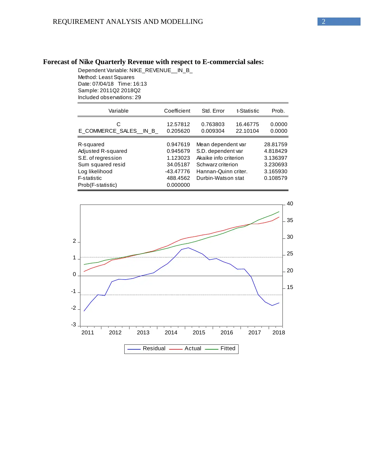
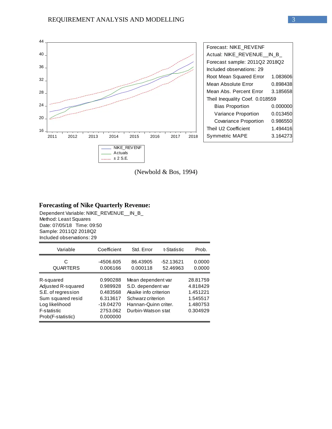
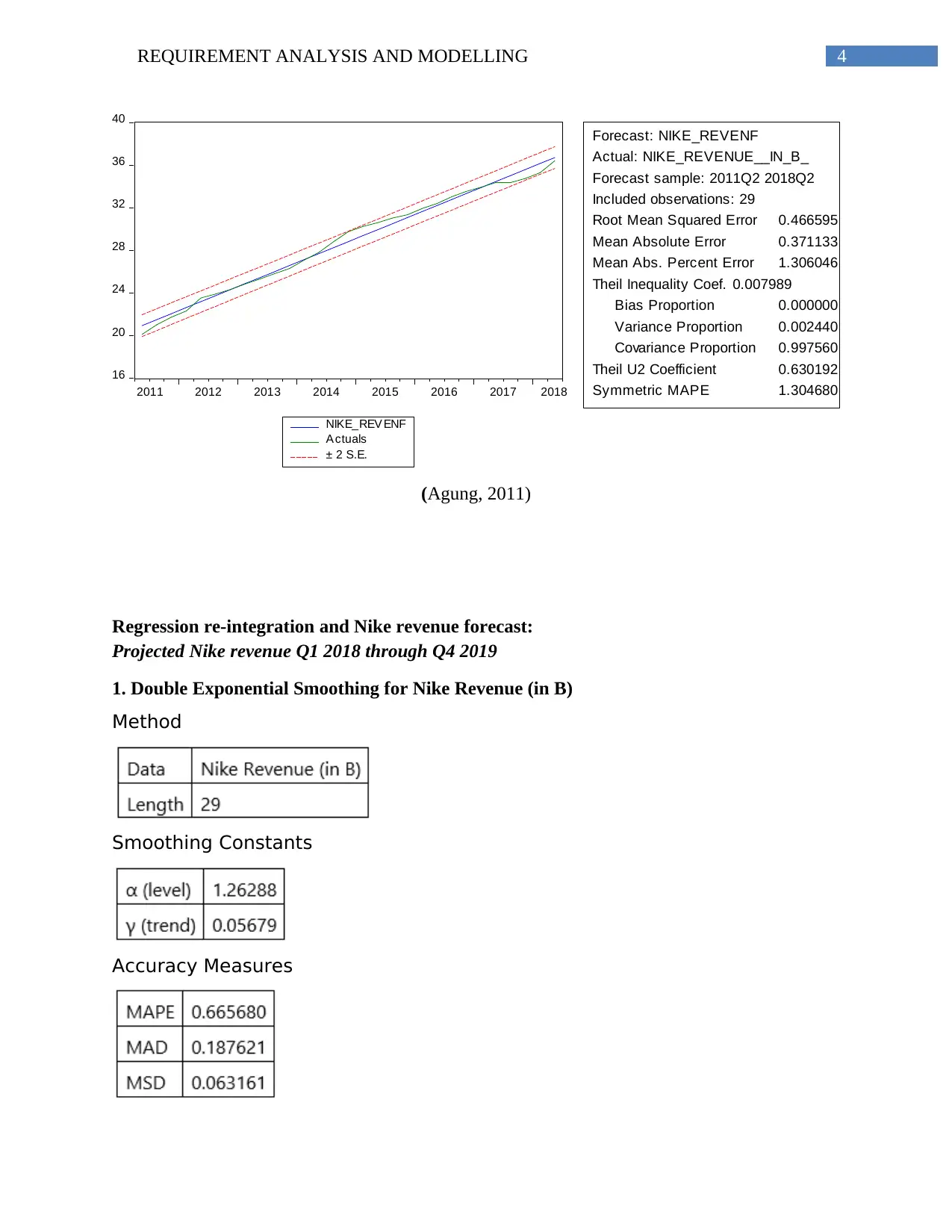
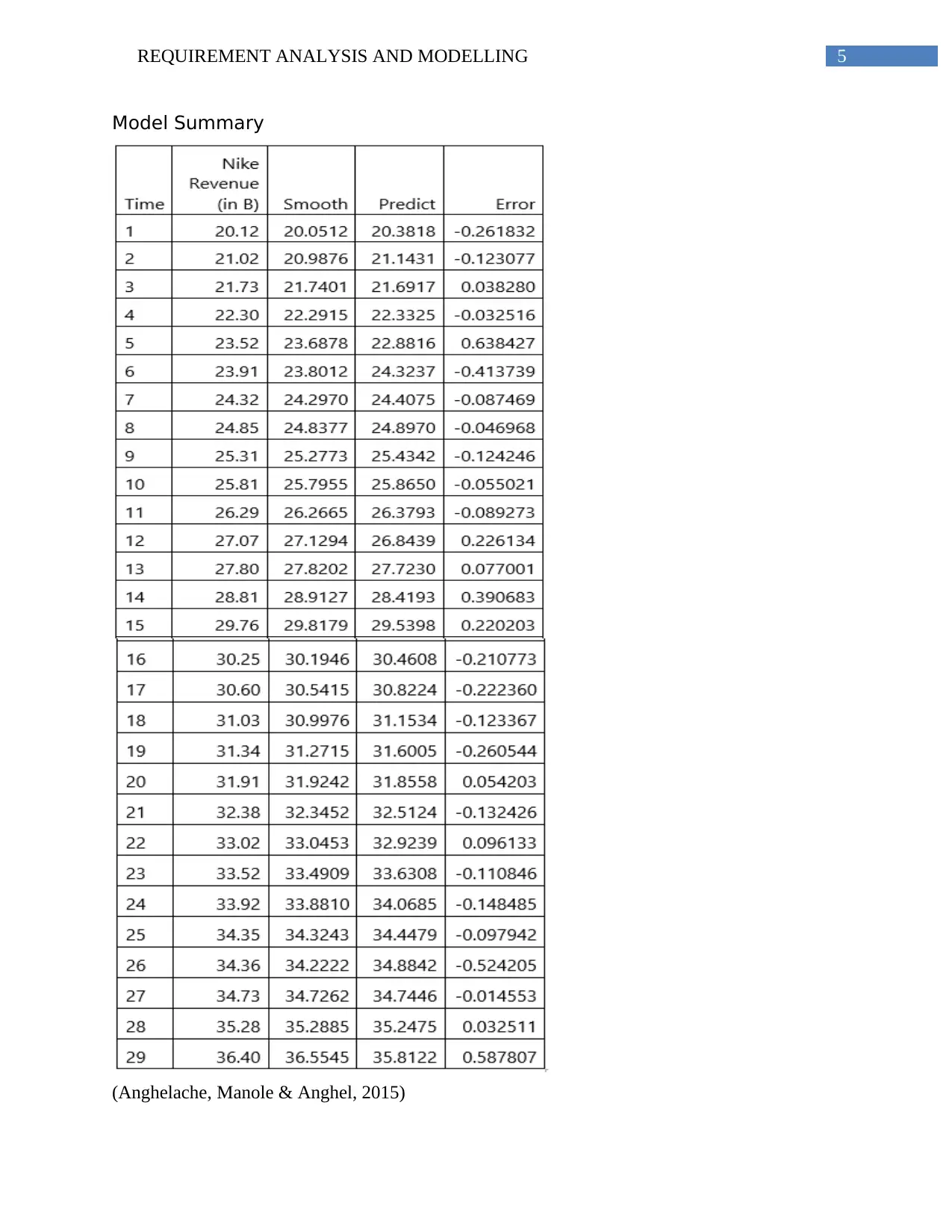
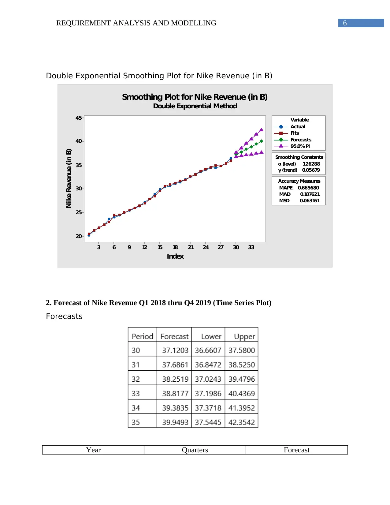
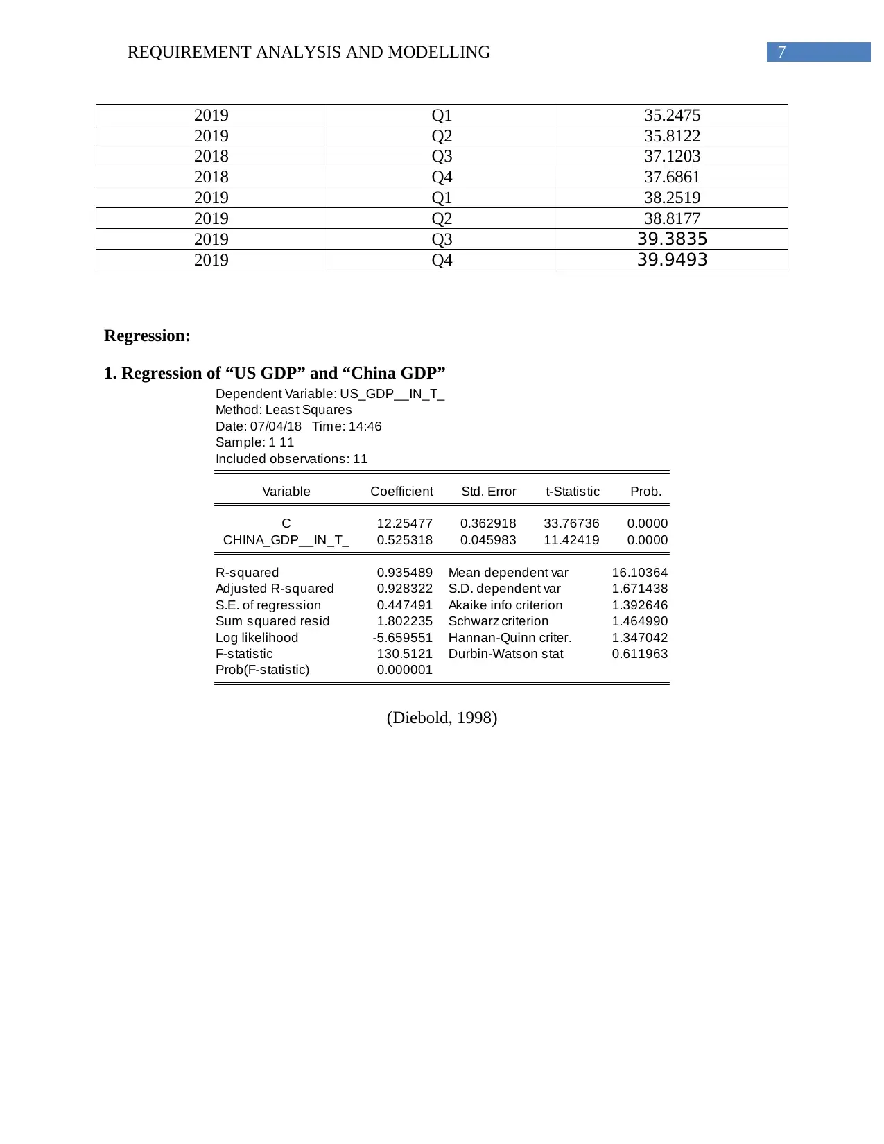
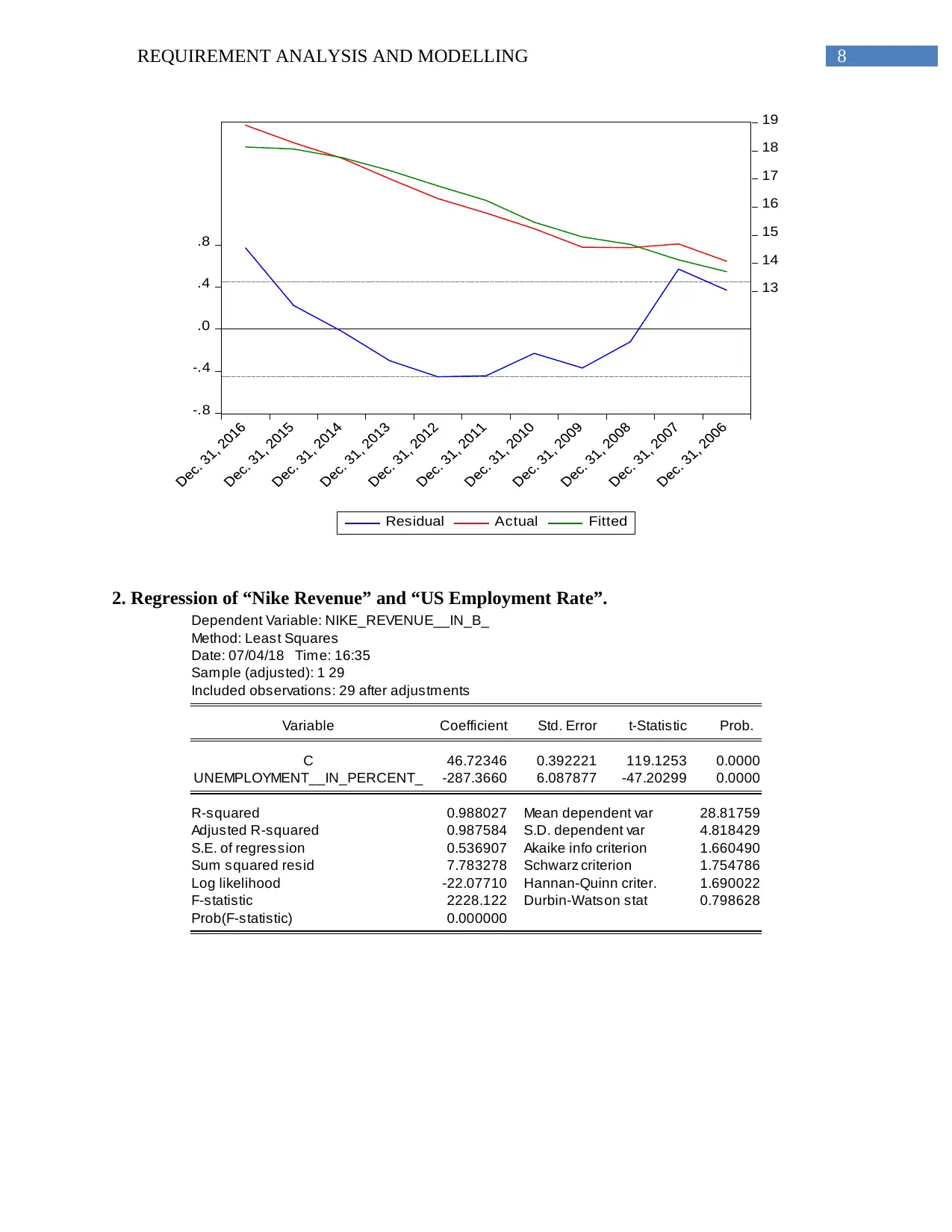
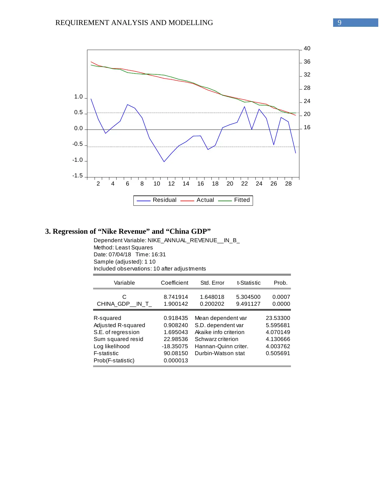
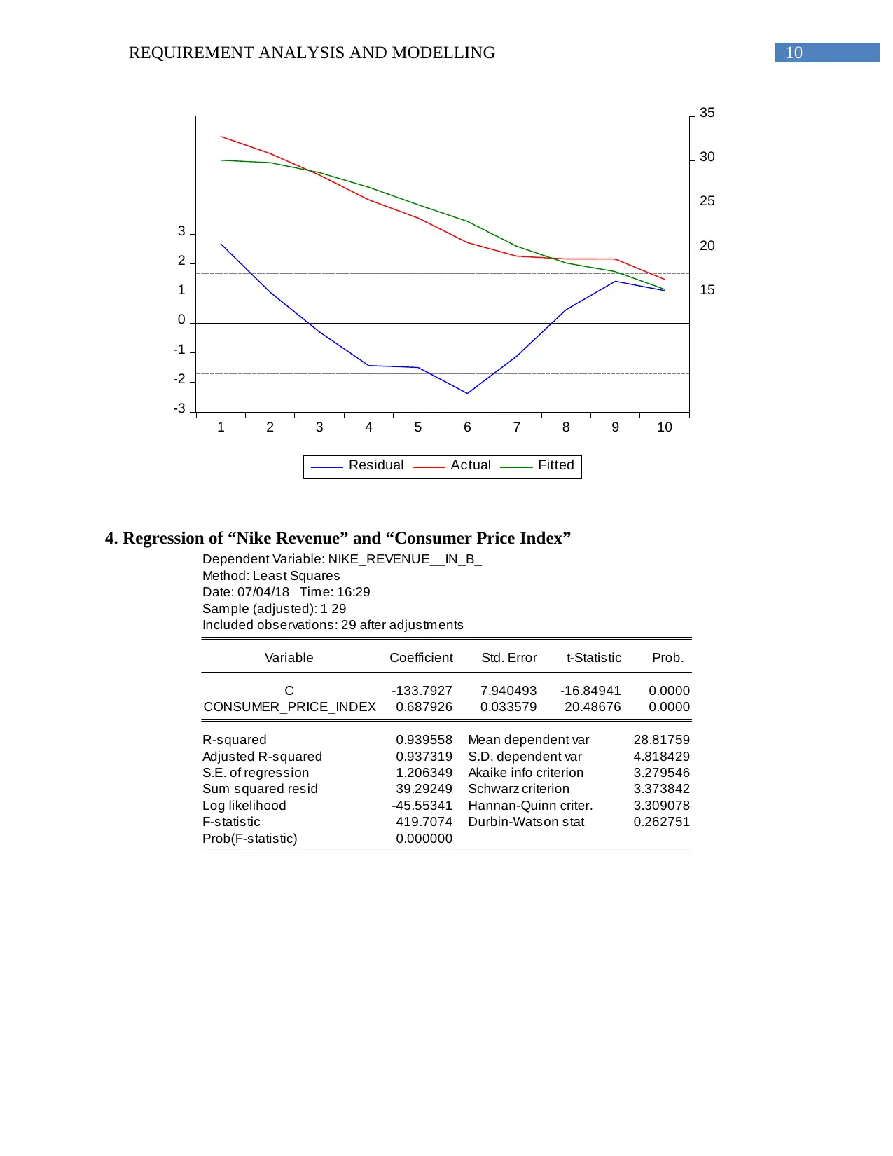
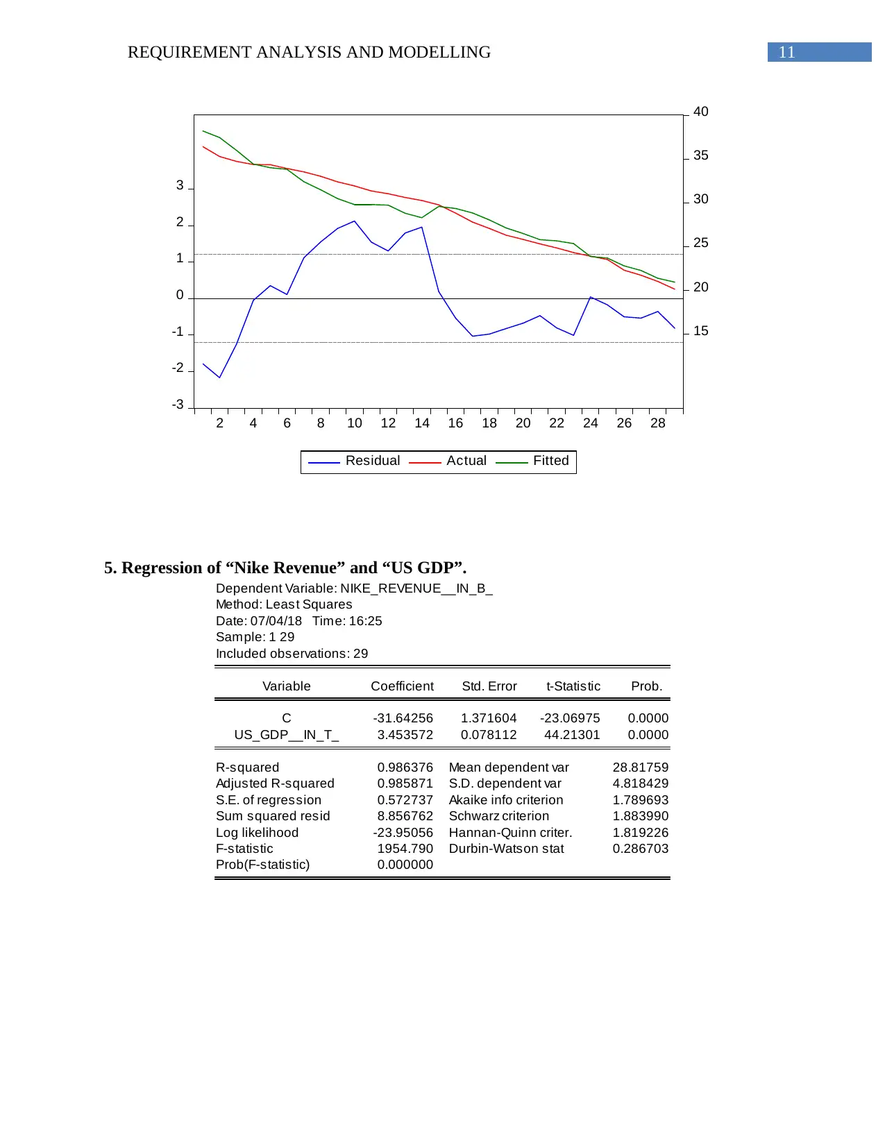
This assignment presents a comprehensive analysis of Nike's quarterly revenue, employing various forecasting and regression techniques. The project begins with an examination of Nike's revenue in relation to e-commerce sales, utilizing least squares regression to establish a correlation. Furthermore, the document explores time series forecasting methods, including double exponential smoothing, to project future revenue. The project delves into multiple regression analyses, assessing the impact of various economic indicators such as US GDP, China GDP, US employment rates, and consumer price indices on Nike's revenue. The analysis includes detailed regression tables, forecast plots, and accuracy measures to validate the models. The report incorporates data from 2011Q2 to 2018Q2 and provides forecasts for Nike's revenue through Q4 2019, offering insights into the relationship between economic factors and the company's financial performance.
1 out of 14
Related Documents


Your All-in-One AI-Powered Toolkit for Academic Success.
+13062052269
info@desklib.com
Available 24*7 on WhatsApp / Email
![[object Object]](/_next/static/media/star-bottom.7253800d.svg)
Copyright © 2020–2025 A2Z Services. All Rights Reserved. Developed and managed by ZUCOL.