Numeracy and Data Analysis

This document provides an in-depth overview of data analysis, including statistical tools such as mean, median, mode, range, and standard deviation. It also covers various chart types and forecasting methods. The content focuses on improving numeracy skills and making informed decisions based on data.

NUMERACY
AND
DATA ANALYSIS

Table of Contents
INTRODUCTION...........................................................................................................................3
MAIN BODY .................................................................................................................................3
1. Data as per the table format ...................................................................................................3
2. Analysing varying forms of charts..........................................................................................3
3. Methodology Used for calculations........................................................................................5
4. Linear forecasting method ......................................................................................................8
CONCLUSION..............................................................................................................................10
REFERENCES..............................................................................................................................11
Books and journals....................................................................................................................11

INTRODUCTION
Data analysis is described as process of performing varying statistical operations which
includes data collection, data interpretation as well as data evaluation. Quantitative data which
also includes survey data, charts and graphs are part of data analysis. It is a procedure which
includes inspection of various useful data in order to arrive at conclusion supporting decision
making process. Data analysis is generally a broad concept, in statistical approach it is classified
into exploratory data analysis, descriptive analysis and so on. Mean, median, mode, range and
standard deviation are statistical tools which are used to evaluate data in order to reach at a
conclusion . Here, we will cover above mentioned tools in order to examine the data by adding
various tables, charts, graphs, etc.
Apart from data analysis, this will include forecasting analysis which means drawing
predictions based over the past as well as present figures and most ordinarily analysis of trends
of the consecutive years (Gallón and Barrientos, 2021).
MAIN BODY
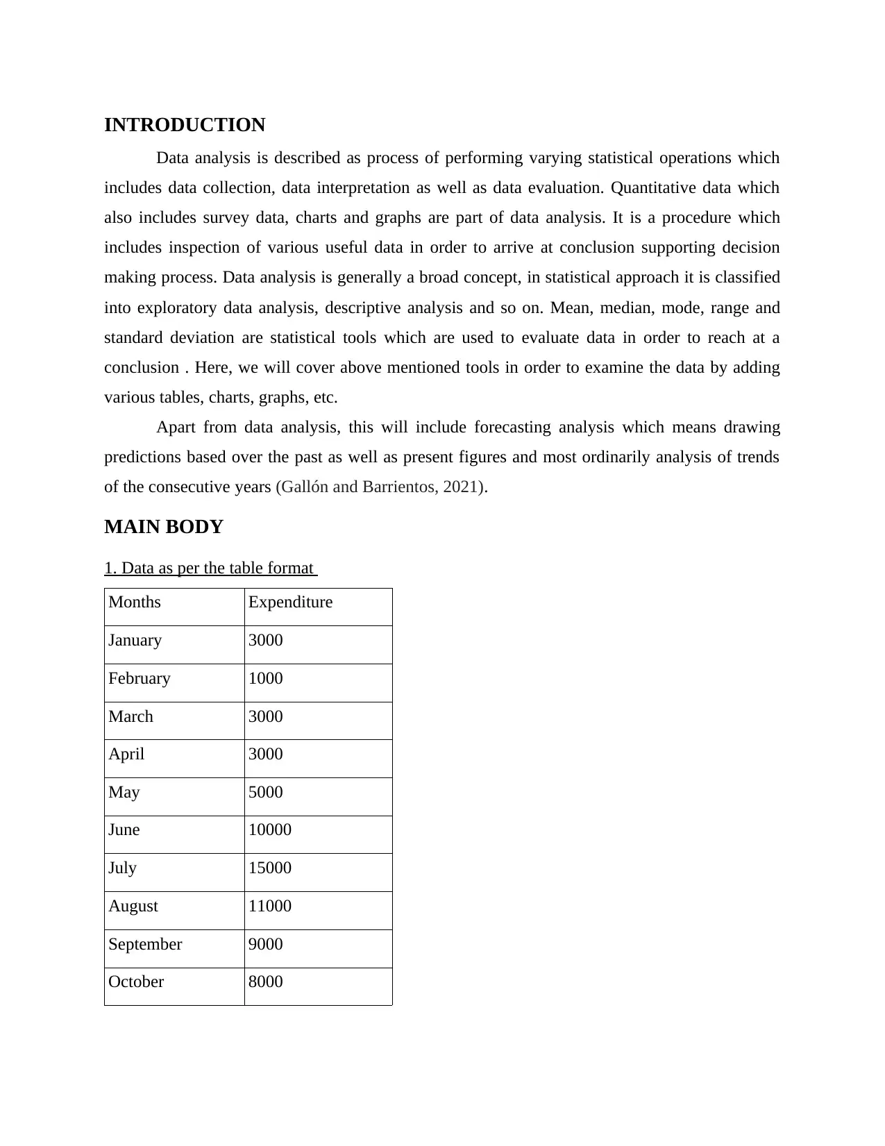
1. Data as per the table format
Months Expenditure
January 3000
February 1000
March 3000
April 3000
May 5000
June 10000
July 15000
August 11000
September 9000
October 8000

2. Analysing varying forms of charts
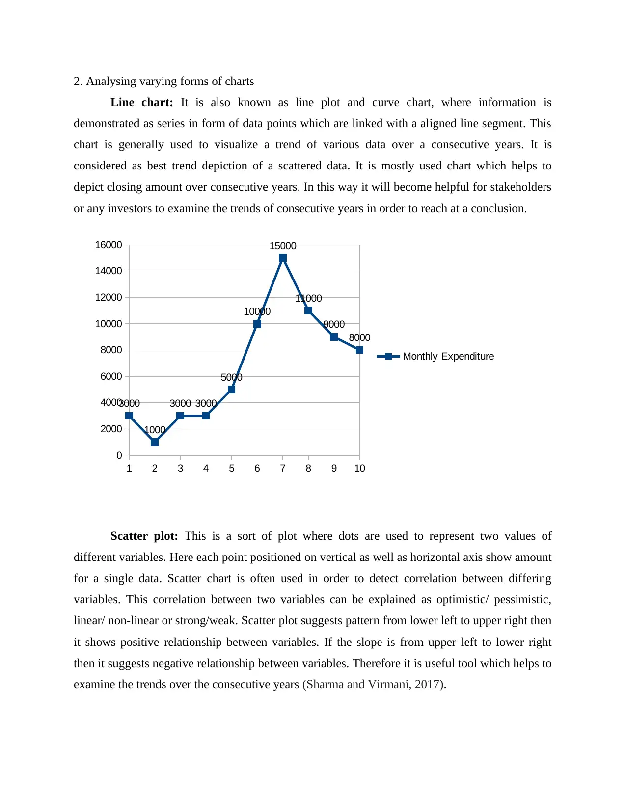
Line chart: It is also known as line plot and curve chart, where information is
demonstrated as series in form of data points which are linked with a aligned line segment. This
chart is generally used to visualize a trend of various data over a consecutive years. It is
considered as best trend depiction of a scattered data. It is mostly used chart which helps to
depict closing amount over consecutive years. In this way it will become helpful for stakeholders
or any investors to examine the trends of consecutive years in order to reach at a conclusion.
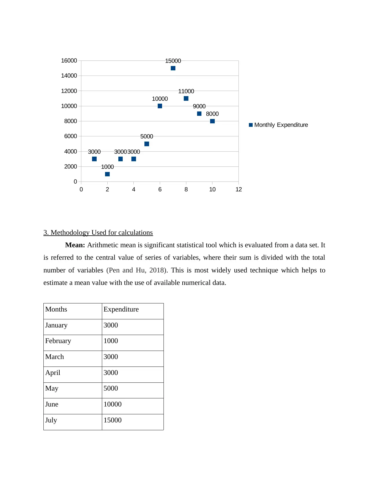
Scatter plot: This is a sort of plot where dots are used to represent two values of
different variables. Here each point positioned on vertical as well as horizontal axis show amount
for a single data. Scatter chart is often used in order to detect correlation between differing
variables. This correlation between two variables can be explained as optimistic/ pessimistic,
linear/ non-linear or strong/weak. Scatter plot suggests pattern from lower left to upper right then
it shows positive relationship between variables. If the slope is from upper left to lower right
then it suggests negative relationship between variables. Therefore it is useful tool which helps to
examine the trends over the consecutive years (Sharma and Virmani, 2017).
1 2 3 4 5 6 7 8 9 10
0
2000
4000
6000
8000
10000
12000
14000
16000
3000
1000
3000 3000
5000
10000
15000
11000
9000
8000
Monthly Expenditure

3. Methodology Used for calculations
Mean: Arithmetic mean is significant statistical tool which is evaluated from a data set. It
is referred to the central value of series of variables, where their sum is divided with the total
number of variables (Pen and Hu, 2018). This is most widely used technique which helps to
estimate a mean value with the use of available numerical data.
Months Expenditure
January 3000
February 1000
March 3000
April 3000
May 5000
June 10000
July 15000
0 2 4 6 8 10 12
0
2000
4000
6000
8000
10000
12000
14000
16000
3000
1000
30003000
5000
10000
15000
11000
9000
8000
Monthly Expenditure

August 11000
September 9000
October 8000
Total 68000
Here, total= 68000
N= 10
Mean= 68000/10= 6800
Median: It is termed as a middle number in ascending or descending or sorted series.
Median is a value which separate lower half of series from higher half in a given distribution,
sample size or population (Berger and Hart, 2020). It is basically used in practical situations such
as bankruptcy, etc. In the given sample size, median will be calculated for consecutive 10
months.
When data set is odd= (N+1)/2th item.
When data set is even= {N/2th item+ N/2th item + 1}2
Months Expenditure
January 3000
February 1000
March 3000
April 3000
May 5000
June 10000
July 15000
August 11000
September 9000
October 8000

Total 68000
Here, N= 10
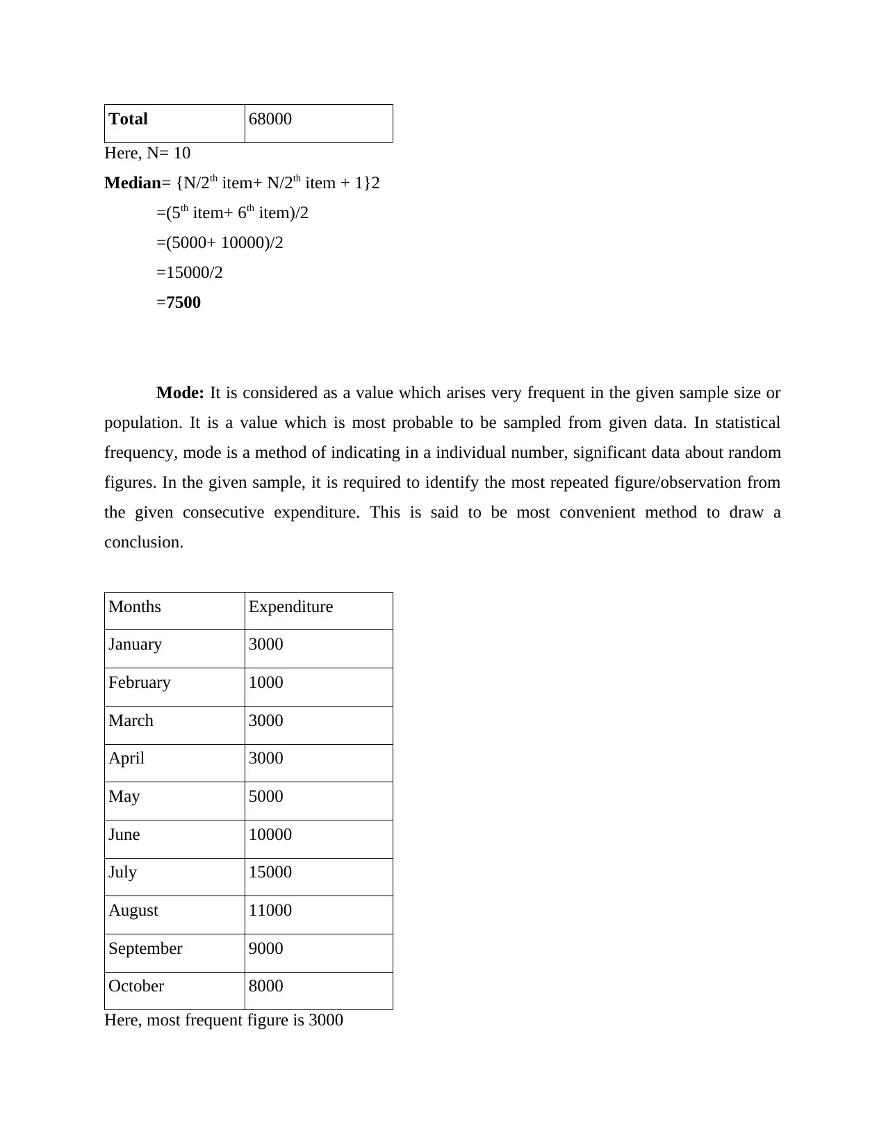
Median= {N/2th item+ N/2th item + 1}2
=(5th item+ 6th item)/2
=(5000+ 10000)/2
=15000/2
=7500
Mode: It is considered as a value which arises very frequent in the given sample size or
population. It is a value which is most probable to be sampled from given data. In statistical
frequency, mode is a method of indicating in a individual number, significant data about random
figures. In the given sample, it is required to identify the most repeated figure/observation from
the given consecutive expenditure. This is said to be most convenient method to draw a
conclusion.
Months Expenditure
January 3000
February 1000
March 3000
April 3000
May 5000
June 10000
July 15000
August 11000
September 9000
October 8000
Here, most frequent figure is 3000

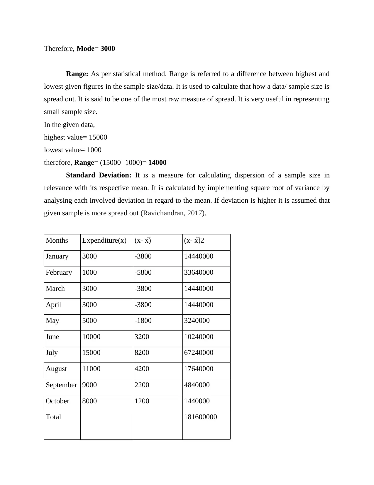
Therefore, Mode= 3000
Range: As per statistical method, Range is referred to a difference between highest and
lowest given figures in the sample size/data. It is used to calculate that how a data/ sample size is
spread out. It is said to be one of the most raw measure of spread. It is very useful in representing
small sample size.
In the given data,
highest value= 15000
lowest value= 1000
therefore, Range= (15000- 1000)= 14000
Standard Deviation: It is a measure for calculating dispersion of a sample size in
relevance with its respective mean. It is calculated by implementing square root of variance by
analysing each involved deviation in regard to the mean. If deviation is higher it is assumed that
given sample is more spread out (Ravichandran, 2017).
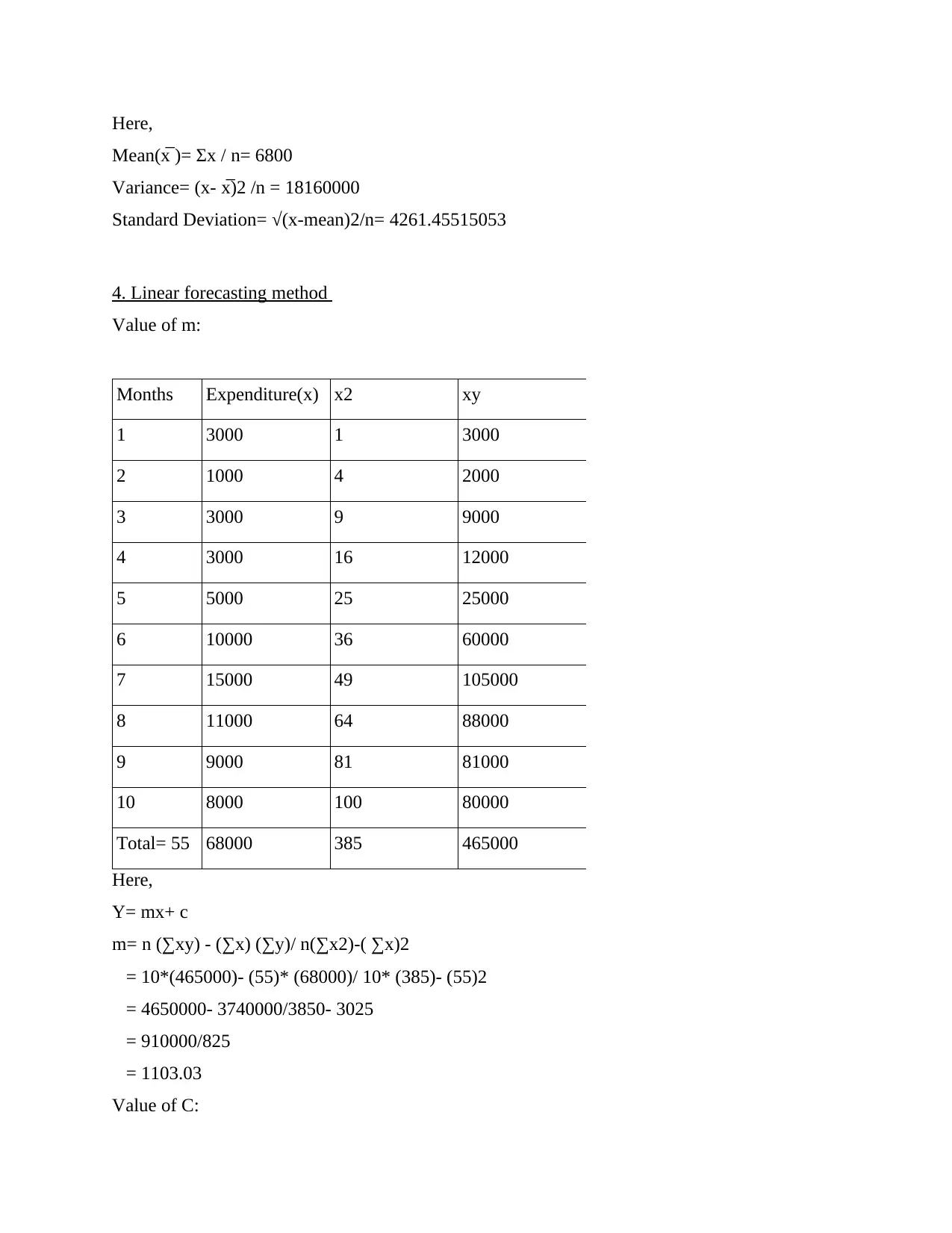
Months Expenditure(x) (x- x̅) (x- x̅)2
January 3000 -3800 14440000
February 1000 -5800 33640000
March 3000 -3800 14440000
April 3000 -3800 14440000
May 5000 -1800 3240000
June 10000 3200 10240000
July 15000 8200 67240000
August 11000 4200 17640000
September 9000 2200 4840000
October 8000 1200 1440000
Total 181600000

Here,
Mean(x̅ )= Σx / n= 6800
Variance= (x- x̅)2 /n = 18160000
Standard Deviation= √(x-mean)2/n= 4261.45515053
4. Linear forecasting method
Value of m:
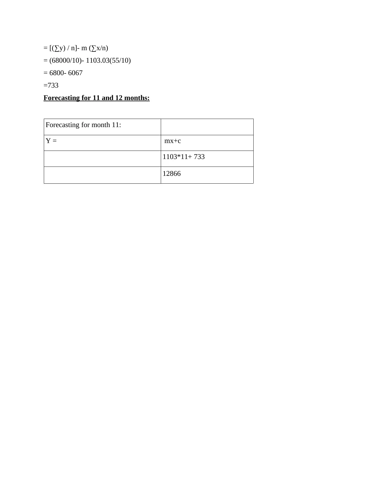
Months Expenditure(x) x2 xy
1 3000 1 3000
2 1000 4 2000
3 3000 9 9000
4 3000 16 12000
5 5000 25 25000
6 10000 36 60000
7 15000 49 105000
8 11000 64 88000
9 9000 81 81000
10 8000 100 80000
Total= 55 68000 385 465000
Here,
Y= mx+ c
m= n (∑xy) - (∑x) (∑y)/ n(∑x2)-( ∑x)2
= 10*(465000)- (55)* (68000)/ 10* (385)- (55)2
= 4650000- 3740000/3850- 3025
= 910000/825
= 1103.03
Value of C:

= [(∑y) / n]- m (∑x/n)
= (68000/10)- 1103.03(55/10)
= 6800- 6067
=733
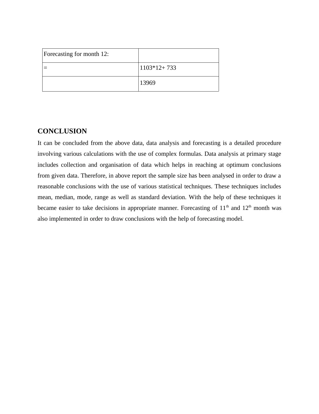
Forecasting for 11 and 12 months:
Forecasting for month 11:
Y = mx+c
1103*11+ 733
12866

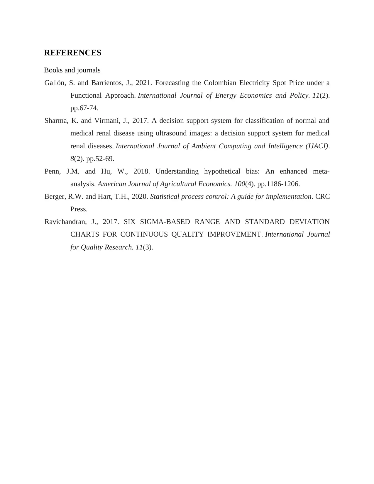
Forecasting for month 12:
= 1103*12+ 733
13969
CONCLUSION
It can be concluded from the above data, data analysis and forecasting is a detailed procedure
involving various calculations with the use of complex formulas. Data analysis at primary stage
includes collection and organisation of data which helps in reaching at optimum conclusions
from given data. Therefore, in above report the sample size has been analysed in order to draw a
reasonable conclusions with the use of various statistical techniques. These techniques includes
mean, median, mode, range as well as standard deviation. With the help of these techniques it
became easier to take decisions in appropriate manner. Forecasting of 11th and 12th month was
also implemented in order to draw conclusions with the help of forecasting model.

REFERENCES
Books and journals
Gallón, S. and Barrientos, J., 2021. Forecasting the Colombian Electricity Spot Price under a
Functional Approach. International Journal of Energy Economics and Policy. 11(2).
pp.67-74.
Sharma, K. and Virmani, J., 2017. A decision support system for classification of normal and
medical renal disease using ultrasound images: a decision support system for medical
renal diseases. International Journal of Ambient Computing and Intelligence (IJACI).
8(2). pp.52-69.
Penn, J.M. and Hu, W., 2018. Understanding hypothetical bias: An enhanced meta-
analysis. American Journal of Agricultural Economics. 100(4). pp.1186-1206.
Berger, R.W. and Hart, T.H., 2020. Statistical process control: A guide for implementation. CRC
Press.
Ravichandran, J., 2017. SIX SIGMA-BASED RANGE AND STANDARD DEVIATION
CHARTS FOR CONTINUOUS QUALITY IMPROVEMENT. International Journal
for Quality Research. 11(3).