Data Analysis Report: Weather Forecasting and Statistical Analysis

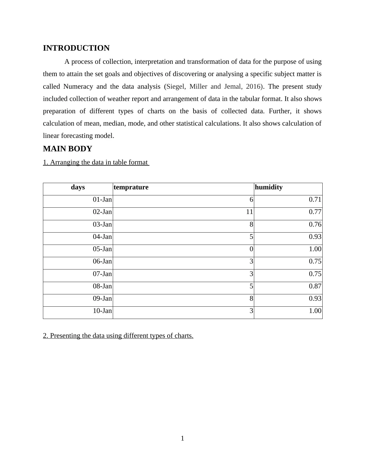
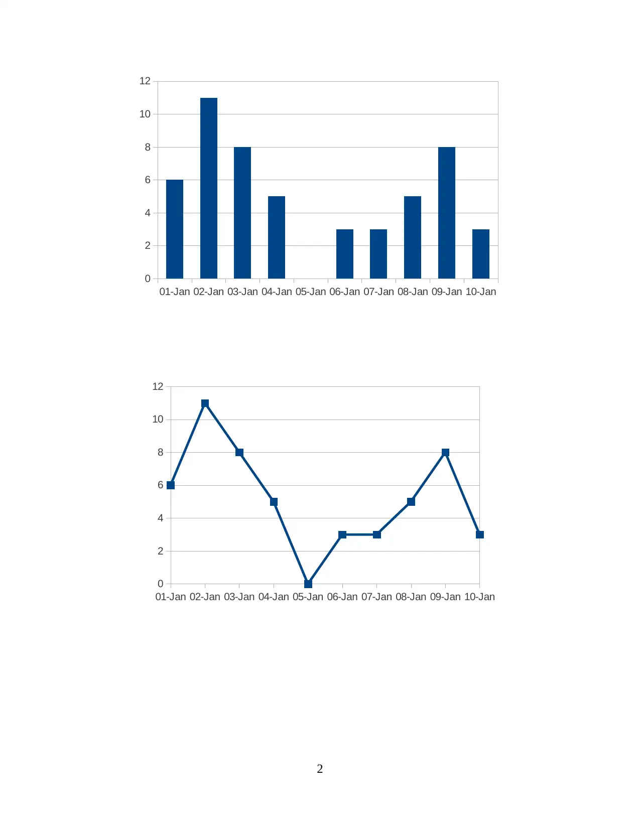
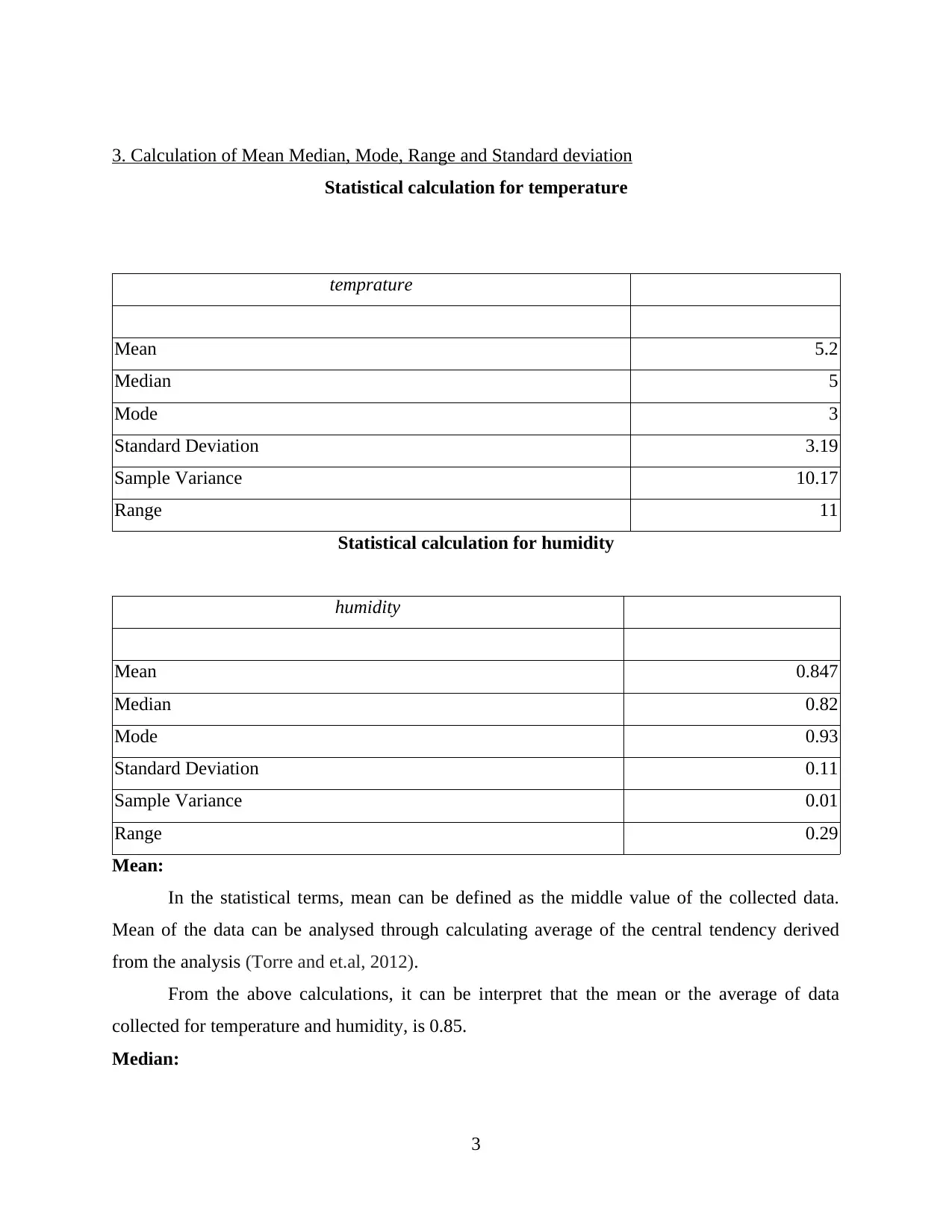
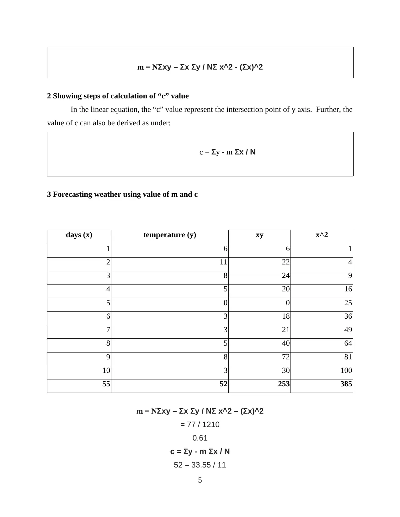
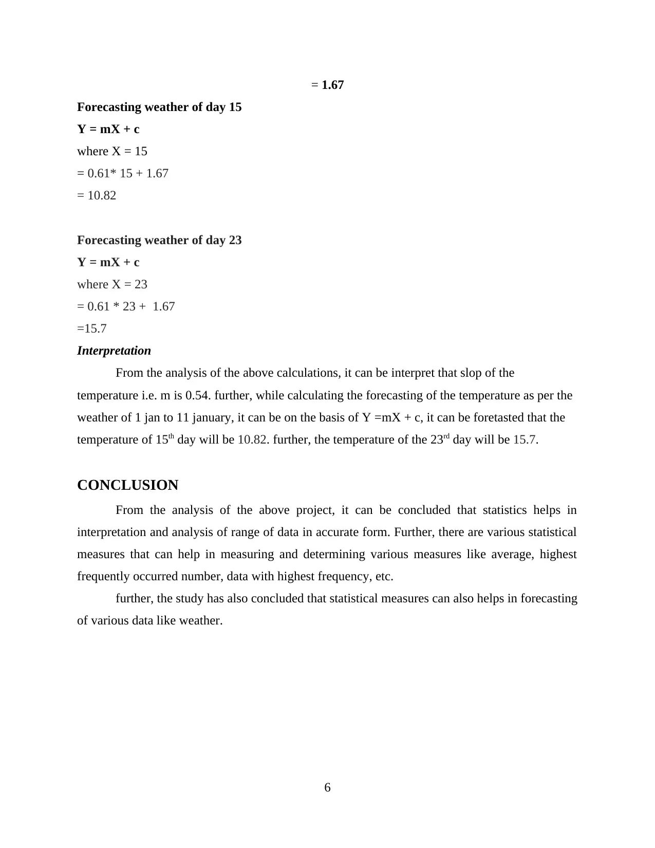
This report provides a comprehensive analysis of weather data, focusing on temperature and humidity. The study begins with arranging the data in a tabular format, followed by the presentation of data using various types of charts. Statistical calculations, including mean, median, mode, range, and standard deviation, are performed to analyze the data. Furthermore, the report incorporates a linear forecasting model to predict future weather patterns. The methodology involves calculating the 'm' and 'c' values of the linear equation and applying these values to forecast temperature for specific days. The conclusion highlights the utility of statistical measures in data interpretation, analysis, and forecasting, emphasizing the application of these techniques to real-world scenarios like weather prediction. The report references several sources, including academic journals and online resources, to support its findings and methodologies.

Numeracy and Data Analysis

Table of Contents
INTRODUCTION...........................................................................................................................1
MAIN BODY...................................................................................................................................1
1. Arranging the data in table format ..........................................................................................1
2. Presenting the data using different types of charts..................................................................1
3. Calculation of Mean Median, Mode, Range and Standard deviation......................................2
4. Presenting statistical calculation using linear forecasting model............................................4
CONCLUSION................................................................................................................................6
REFERENCES................................................................................................................................7

INTRODUCTION
A process of collection, interpretation and transformation of data for the purpose of using
them to attain the set goals and objectives of discovering or analysing a specific subject matter is
called Numeracy and the data analysis (Siegel, Miller and Jemal, 2016). The present study
included collection of weather report and arrangement of data in the tabular format. It also shows
preparation of different types of charts on the basis of collected data. Further, it shows
calculation of mean, median, mode, and other statistical calculations. It also shows calculation of
linear forecasting model.
MAIN BODY
1. Arranging the data in table format
days temprature humidity
01-Jan 6 0.71
02-Jan 11 0.77
03-Jan 8 0.76
04-Jan 5 0.93
05-Jan 0 1.00
06-Jan 3 0.75
07-Jan 3 0.75
08-Jan 5 0.87
09-Jan 8 0.93
10-Jan 3 1.00
2. Presenting the data using different types of charts.
1

2
01-Jan 02-Jan 03-Jan 04-Jan 05-Jan 06-Jan 07-Jan 08-Jan 09-Jan 10-Jan
0
2
4
6
8
10
12
01-Jan 02-Jan 03-Jan 04-Jan 05-Jan 06-Jan 07-Jan 08-Jan 09-Jan 10-Jan
0
2
4
6
8
10
12

3. Calculation of Mean Median, Mode, Range and Standard deviation
Statistical calculation for temperature
temprature
Mean 5.2
Median 5
Mode 3
Standard Deviation 3.19
Sample Variance 10.17
Range 11
Statistical calculation for humidity
humidity
Mean 0.847
Median 0.82
Mode 0.93
Standard Deviation 0.11
Sample Variance 0.01
Range 0.29
Mean:
In the statistical terms, mean can be defined as the middle value of the collected data.
Mean of the data can be analysed through calculating average of the central tendency derived
from the analysis (Torre and et.al, 2012).
From the above calculations, it can be interpret that the mean or the average of data
collected for temperature and humidity, is 0.85.
Median:
3

The median of the statistical data shows the middle most value of the collected or
observed data. For the purpose of determination of median, the overall data is needed to be
arranged in the chronological order (Znamenskiy and et.al., 2018). In this order, the middle most
value of the central tendency can be derived in an effective manner.
The median of the observed data came 0.87. therefore, it can be analysed that the middle
most value the collected data regarding humidity. Further, the middle most value of the observed
data related to temperature has been derived to 5.
Mode:
Mode is the process of determining the most frequent number or data of the observation.
While calculating the mode, frequency of the each collected data is determined. The most
frequently occurred data is termed as the mode of observed data.
In the present collected data, the most frequent data in the temperature has been observed
to be 3. on the other hand, in the collected data regarding the humidity, the observed mode is
0.93.
Range
In the statistical term, the difference between highest and the lowest value of the set of
collected data is known as range (Pravilovic and et.al., 2017).
The difference between the highest and lowest lowest value of the temperature is 11. in
addition, the range of the humidity is 0.29.
Standard Deviation
Standard deviation shows the variation in the observed set of data in the quantitative term
(Beydoun and et.al., 2016). In other words, standard deviation can be defined as the dispersion
of the data is derived by square rooting the variation of the set.
The variation in the observed data of temperature is 3.07. on the other hand, the vairation
in the humidity data is being observed to be 0.11.
4. Presenting statistical calculation using linear forecasting model
1 Showing steps to calculate “m” value
In the linear equation y = mx + c, “m” shows the slope. In this regard, the calculation of
“m” value can be analysed as under:
4

m = NΣxy – Σx Σy / NΣ x^2 - (Σx)^2
2 Showing steps of calculation of “c” value
In the linear equation, the “c” value represent the intersection point of y axis. Further, the
value of c can also be derived as under:
c = Σy - m Σx / N
3 Forecasting weather using value of m and c
days (x) temperature (y) xy x^2
1 6 6 1
2 11 22 4
3 8 24 9
4 5 20 16
5 0 0 25
6 3 18 36
7 3 21 49
8 5 40 64
9 8 72 81
10 3 30 100
55 52 253 385
m = NΣxy – Σx Σy / NΣ x^2 – (Σx)^2
= 77 / 1210
0.61
c = Σy - m Σx / N
52 – 33.55 / 11
5

= 1.67
Forecasting weather of day 15
Y = mX + c
where X = 15
= 0.61* 15 + 1.67
= 10.82
Forecasting weather of day 23
Y = mX + c
where X = 23
= 0.61 * 23 + 1.67
=15.7
Interpretation
From the analysis of the above calculations, it can be interpret that slop of the
temperature i.e. m is 0.54. further, while calculating the forecasting of the temperature as per the
weather of 1 jan to 11 january, it can be on the basis of Y =mX + c, it can be foretasted that the
temperature of 15th day will be 10.82. further, the temperature of the 23rd day will be 15.7.
CONCLUSION
From the analysis of the above project, it can be concluded that statistics helps in
interpretation and analysis of range of data in accurate form. Further, there are various statistical
measures that can help in measuring and determining various measures like average, highest
frequently occurred number, data with highest frequency, etc.
further, the study has also concluded that statistical measures can also helps in forecasting
of various data like weather.
6

REFERENCES
Books and Journals
Siegel, R. L., Miller, K. D. and Jemal, A., 2016. Cancer statistics, 2016. CA: a cancer journal for
clinicians. 66(1). pp.7-30.
Torre, L.A. and et.al, 2012. CA: a cancer journal for clinicians, 65(2), pp.87-108.
Znamenskiy, P. and et.al., 2018. Functional selectivity and specific connectivity of inhibitory
neurons in primary visual cortex. bioRxiv, p.294835.
Pravilovic, S. and et.al., 2017. Using multiple time series analysis for geosensor data
forecasting. Information Sciences. 380. pp.31-52.
Beydoun, M.A. and et.al., 2016. Racial disparities in adult all-cause and cause-specific mortality
among us adults: mediating and moderating factors. BMC public health. 16(1). p.1113.
Online
[Online] Available through : <https://towardsdatascience.com/mathematics-for-machine-
learning-linear-regression-least-square-regression-de09cf53757c>
7