Numeracy and Data Analysis
VerifiedAdded on 2023/01/12
|10
|1437
|1
AI Summary
This report provides insights into numeracy and data analysis, focusing on presenting data, graphical presentation, descriptive statistics, and forecasting using the linear method. It explores the weather conditions in Lewisham, London.
Contribute Materials
Your contribution can guide someone’s learning journey. Share your
documents today.
Numeracy and Data
Analysis
Analysis
Secure Best Marks with AI Grader
Need help grading? Try our AI Grader for instant feedback on your assignments.
Table of Contents
INTRODUCTION......................................................................................................................3
1. Presenting the data.............................................................................................................3
2. Graphical presentation of data set......................................................................................3
3. Descriptive statistics...........................................................................................................4
4. Presenting the forecast by using linear method..................................................................7
CONCLUSION..........................................................................................................................9
REFERENCES.........................................................................................................................10
INTRODUCTION
Data analysis is the set of statistical tools and techniques which in turn assist to
determine the facts and figures. The tool are highly important because it will assist to
evaluate the present as well as forecasting about future. Thus, for this report, Lewisham of
London is selected and provide insight about complete weather condition.
1. Presenting the data
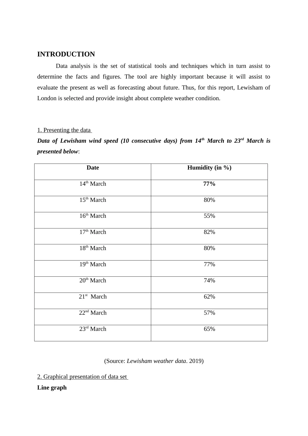
Data of Lewisham wind speed (10 consecutive days) from 14th March to 23rd March is
presented below:
Date Humidity (in %)
14th March 77%
15th March 80%
16th March 55%
17th March 82%
18th March 80%
19th March 77%
20th March 74%
21st March 62%
22nd March 57%
23rd March 65%
(Source: Lewisham weather data. 2019)
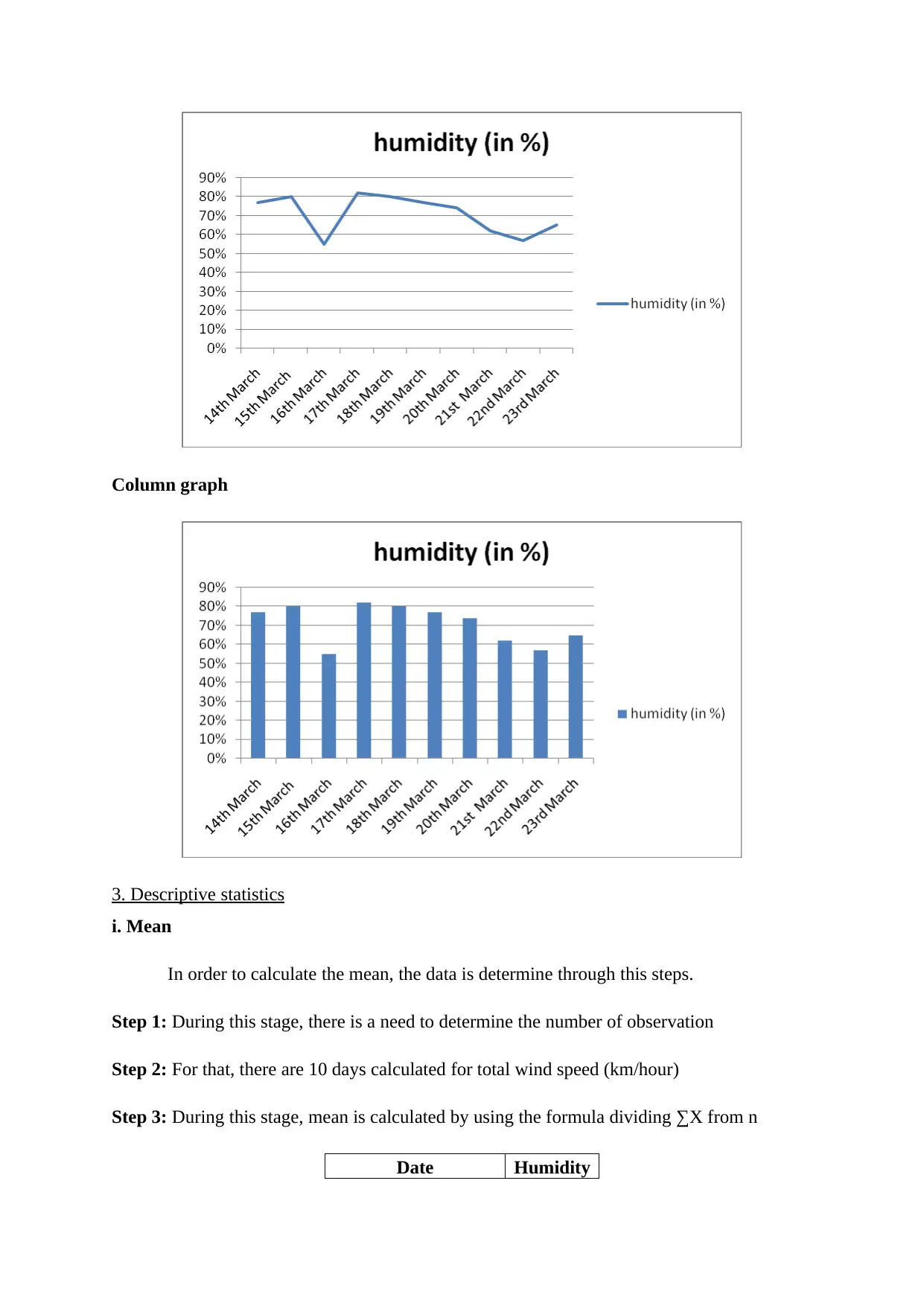
2. Graphical presentation of data set
Line graph
Column graph
3. Descriptive statistics
i. Mean
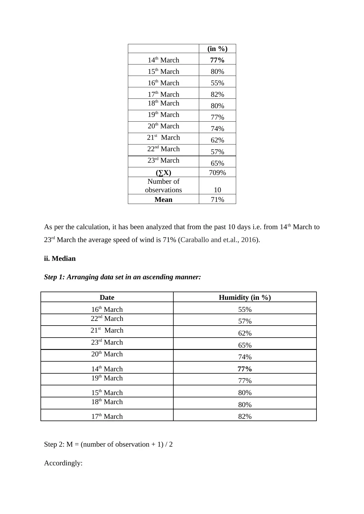
In order to calculate the mean, the data is determine through this steps.
Step 1: During this stage, there is a need to determine the number of observation
Step 2: For that, there are 10 days calculated for total wind speed (km/hour)
Step 3: During this stage, mean is calculated by using the formula dividing ∑X from n
Date Humidity
Paraphrase This Document
Need a fresh take? Get an instant paraphrase of this document with our AI Paraphraser
(in %)
14th March 77%
15th March 80%
16th March 55%
17th March 82%
18th March 80%
19th March 77%
20th March 74%
21st March 62%
22nd March 57%
23rd March 65%
(∑X) 709%
Number of
observations 10
Mean 71%
As per the calculation, it has been analyzed that from the past 10 days i.e. from 14th March to
23rd March the average speed of wind is 71% (Caraballo and et.al., 2016).
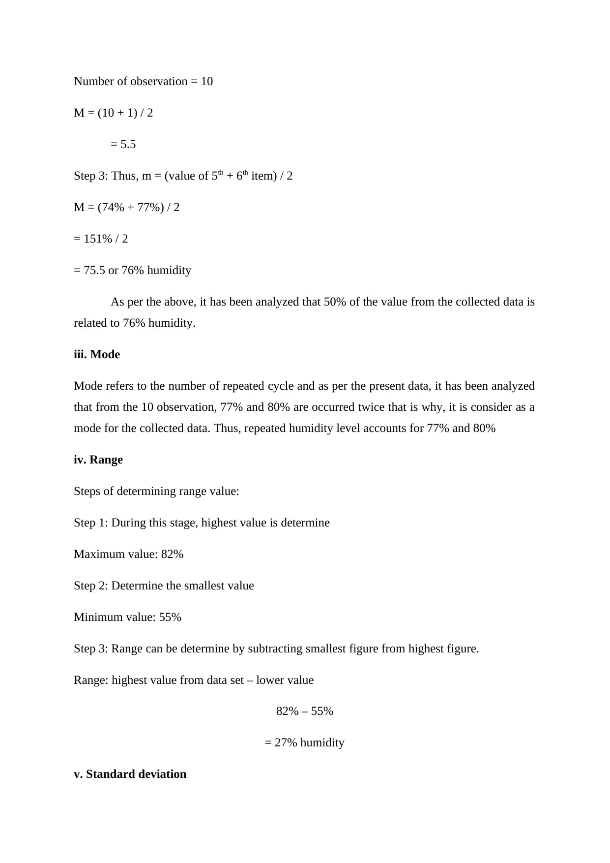
ii. Median
Step 1: Arranging data set in an ascending manner:
Date Humidity (in %)
16th March 55%
22nd March 57%
21st March 62%
23rd March 65%
20th March 74%
14th March 77%
19th March 77%
15th March 80%
18th March 80%
17th March 82%
Step 2: M = (number of observation + 1) / 2
Accordingly:
14th March 77%
15th March 80%
16th March 55%
17th March 82%
18th March 80%
19th March 77%
20th March 74%
21st March 62%
22nd March 57%
23rd March 65%
(∑X) 709%
Number of
observations 10
Mean 71%
As per the calculation, it has been analyzed that from the past 10 days i.e. from 14th March to
23rd March the average speed of wind is 71% (Caraballo and et.al., 2016).
ii. Median
Step 1: Arranging data set in an ascending manner:
Date Humidity (in %)
16th March 55%
22nd March 57%
21st March 62%
23rd March 65%
20th March 74%
14th March 77%
19th March 77%
15th March 80%
18th March 80%
17th March 82%
Step 2: M = (number of observation + 1) / 2
Accordingly:
Number of observation = 10
M = (10 + 1) / 2
= 5.5
Step 3: Thus, m = (value of 5th + 6th item) / 2
M = (74% + 77%) / 2
= 151% / 2
= 75.5 or 76% humidity
As per the above, it has been analyzed that 50% of the value from the collected data is
related to 76% humidity.
iii. Mode
Mode refers to the number of repeated cycle and as per the present data, it has been analyzed
that from the 10 observation, 77% and 80% are occurred twice that is why, it is consider as a
mode for the collected data. Thus, repeated humidity level accounts for 77% and 80%
iv. Range
Steps of determining range value:
Step 1: During this stage, highest value is determine
Maximum value: 82%
Step 2: Determine the smallest value
Minimum value: 55%
Step 3: Range can be determine by subtracting smallest figure from highest figure.
Range: highest value from data set – lower value
82% – 55%
= 27% humidity
v. Standard deviation
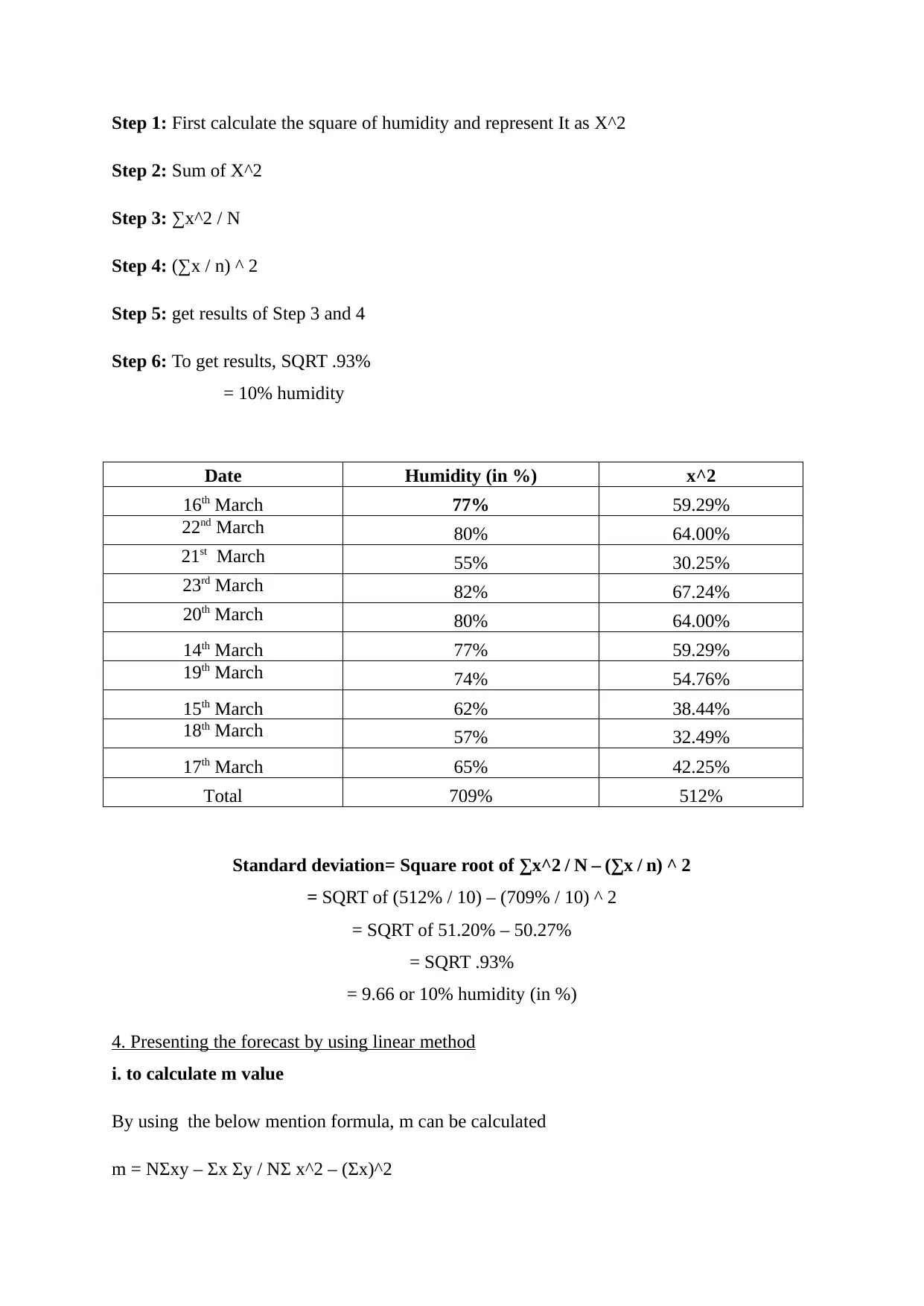
Step 1: First calculate the square of humidity and represent It as X^2
Step 2: Sum of X^2
Step 3: ∑x^2 / N
Step 4: (∑x / n) ^ 2
Step 5: get results of Step 3 and 4
Step 6: To get results, SQRT .93%
= 10% humidity
Date Humidity (in %) x^2
16th March 77% 59.29%
22nd March 80% 64.00%
21st March 55% 30.25%
23rd March 82% 67.24%
20th March 80% 64.00%
14th March 77% 59.29%
19th March 74% 54.76%
15th March 62% 38.44%
18th March 57% 32.49%
17th March 65% 42.25%
Total 709% 512%
Standard deviation= Square root of ∑x^2 / N – (∑x / n) ^ 2
= SQRT of (512% / 10) – (709% / 10) ^ 2
= SQRT of 51.20% – 50.27%
= SQRT .93%
= 9.66 or 10% humidity (in %)
4. Presenting the forecast by using linear method
i. to calculate m value
By using the below mention formula, m can be calculated
m = NΣxy – Σx Σy / NΣ x^2 – (Σx)^2
Secure Best Marks with AI Grader
Need help grading? Try our AI Grader for instant feedback on your assignments.
1. Under the first stage, Σxy is multiplied by n
2. Then multiplication of Σx* Σy by n
3. Then formula is used i.e. NΣxy – Σx Σy
4. Then, NΣ x^2 – (Σx)^2
5. Results are generated by NΣxy – Σx Σy / NΣ x^2 – (Σx)^2 (Barbic, Borgioli and
Klacso, 2017)
ii. For calculating c
1. Summation of Y is determines. Here Y = humidity
2. Next step, M * ΣX the formula is used
3. Them the value of m * Σx is divided by n
4. Step 3 is subtracted from Σy
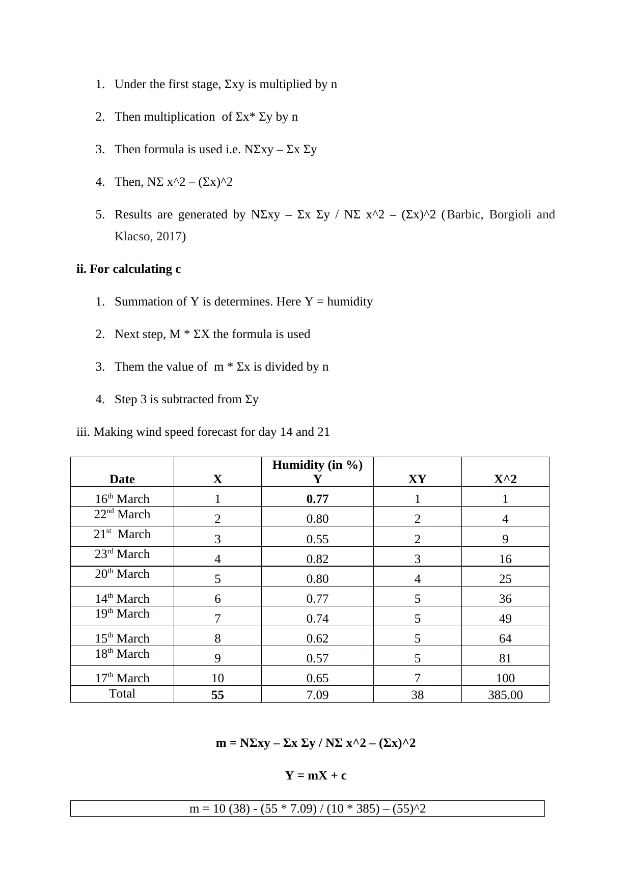
iii. Making wind speed forecast for day 14 and 21
Date X
Humidity (in %)
Y XY X^2
16th March 1 0.77 1 1
22nd March 2 0.80 2 4
21st March 3 0.55 2 9
23rd March 4 0.82 3 16
20th March 5 0.80 4 25
14th March 6 0.77 5 36
19th March 7 0.74 5 49
15th March 8 0.62 5 64
18th March 9 0.57 5 81
17th March 10 0.65 7 100
Total 55 7.09 38 385.00
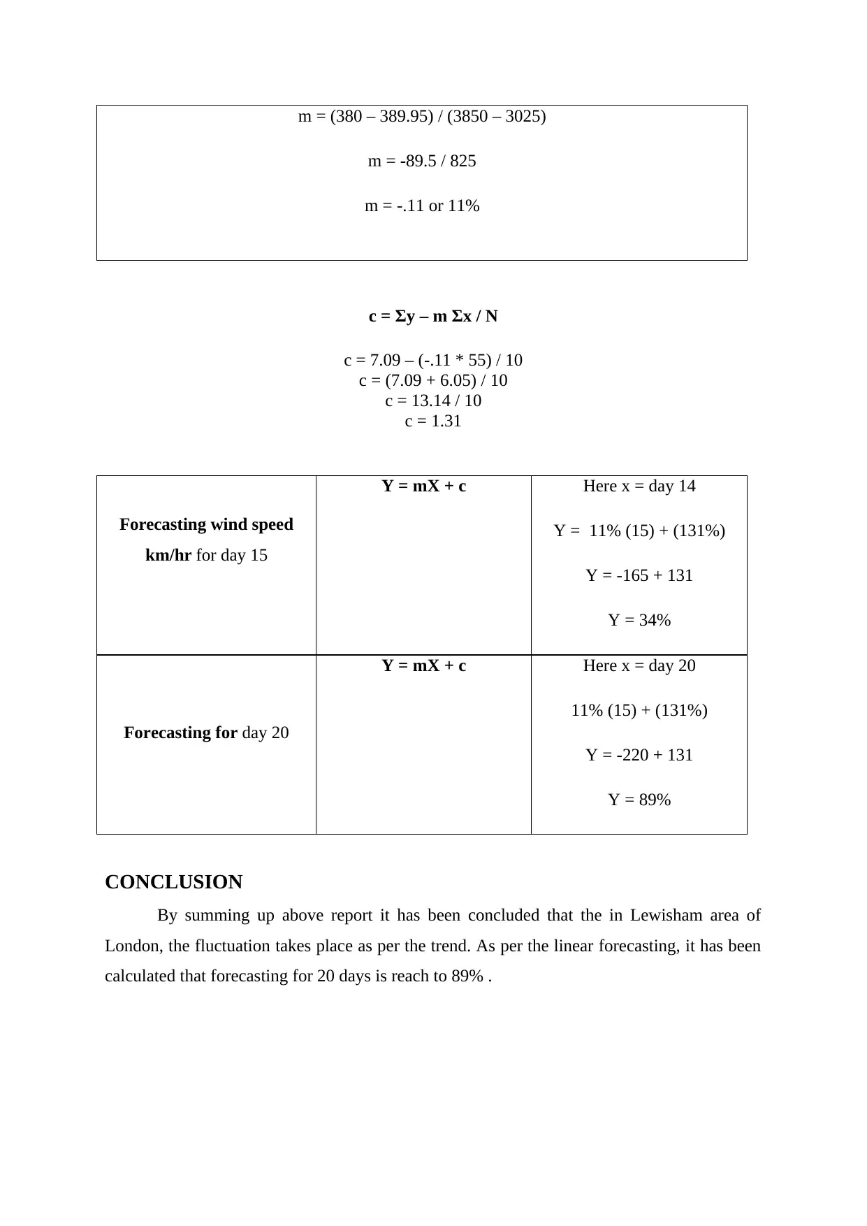
m = NΣxy – Σx Σy / NΣ x^2 – (Σx)^2
Y = mX + c
m = 10 (38) - (55 * 7.09) / (10 * 385) – (55)^2
m = (380 – 389.95) / (3850 – 3025)
m = -89.5 / 825
m = -.11 or 11%
c = Σy – m Σx / N
c = 7.09 – (-.11 * 55) / 10
c = (7.09 + 6.05) / 10
c = 13.14 / 10
c = 1.31
Forecasting wind speed
km/hr for day 15
Y = mX + c Here x = day 14
Y = 11% (15) + (131%)
Y = -165 + 131
Y = 34%
Forecasting for day 20
Y = mX + c Here x = day 20
11% (15) + (131%)
Y = -220 + 131
Y = 89%
CONCLUSION
By summing up above report it has been concluded that the in Lewisham area of
London, the fluctuation takes place as per the trend. As per the linear forecasting, it has been
calculated that forecasting for 20 days is reach to 89% .
REFERENCES
Books and Journals
Barbic, G., Borgioli, S. and Klacso, J., 2017. The journey from micro supervisory data to
aggregate macroprudential statictics (No. 20). ECB Statistics Paper.
Caraballo, A. A. M. and et.al., 2016, November. Automatic creation and analysis of a linked
data cloud diagram. In International Conference on Web Information Systems
Engineering (pp. 417-432). Springer, Cham.
Online
Lewisham weather data. 2020. Online. Available through: <
https://www.worldweatheronline.com/lewisham-weather-history/lewisham-greater-
london/gb.aspx >.
1 out of 10
Related Documents
Your All-in-One AI-Powered Toolkit for Academic Success.
+13062052269
info@desklib.com
Available 24*7 on WhatsApp / Email
Unlock your academic potential
© 2024 | Zucol Services PVT LTD | All rights reserved.