The Assignment on Nursing Statistics

Running head: NURSING STATISTICS
Nursing Statistics
Name of the Student
Name of the University
Author note

1NURSING STATISTICS
Question #1
With the increment of the sample size confidence interval range becomes smaller, or the level
of confidence increases for a chosen range of mean. This probability estimation is true for
normal distribution.
For conducting same study twice with sample of n=500 and n=1000, the second study with
n=1000 will determine better association than the first study, because of the low confidence
interval range for a chosen level of confidence.
The relation of confidence interval with the standard deviation is CI=M±(z*SD/sqrtN), where
M is the mean value of the sample, z is the normal distribution length on x-axis and SD is
standard deviation. Therefore, it can be seen that with the higher value of N, the value
(z*SD/sqrtN) will be less and therefore the plus-minus adjustment with mean value will be
reduce. The square-root of sample size is related with the Confidence Interval.
Question 2
a)
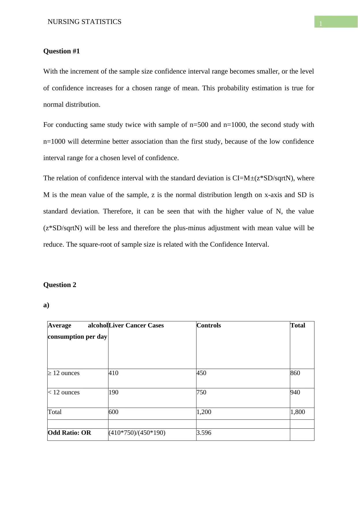
Average alcohol
consumption per day
Liver Cancer Cases Controls Total
≥ 12 ounces 410 450 860
< 12 ounces 190 750 940
Total 600 1,200 1,800
Odd Ratio: OR (410*750)/(450*190) 3.596

2NURSING STATISTICS
In the above case control study to find the association between alcohol consumption and liver
cancer, it has been found that the odd ratio is approximately 3.6. The OR value is much
higher than the probability testing value 1 and therefore it indicates that people who drinks
more than 12 ounces alcohol per day has much higher chances of suffering from liver cancer
than the people who drink less.
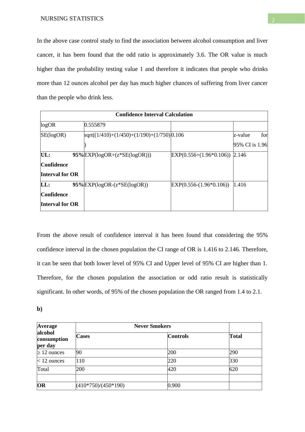
Confidence Interval Calculation
logOR 0.555879
SE(logOR) sqrt((1/410)+(1/450)+(1/190)+(1/750)
)
0.106 z-value for
95% CI is 1.96
UL: 95%
Confidence
Interval for OR
EXP(logOR+(z*SE(logOR))) EXP(0.556+(1.96*0.106)) 2.146
LL: 95%
Confidence
Interval for OR
EXP(logOR-(z*SE(logOR)) EXP(0.556-(1.96*0.106)) 1.416
From the above result of confidence interval it has been found that considering the 95%
confidence interval in the chosen population the CI range of OR is 1.416 to 2.146. Therefore,
it can be seen that both lower level of 95% CI and Upper level of 95% CI are higher than 1.
Therefore, for the chosen population the association or odd ratio result is statistically
significant. In other words, of 95% of the chosen population the OR ranged from 1.4 to 2.1.
b)
Average
alcohol
consumption
per day
Never Smokers
Cases Controls Total
≥ 12 ounces 90 200 290
< 12 ounces 110 220 330
Total 200 420 620
OR (410*750)/(450*190) 0.900

3NURSING STATISTICS
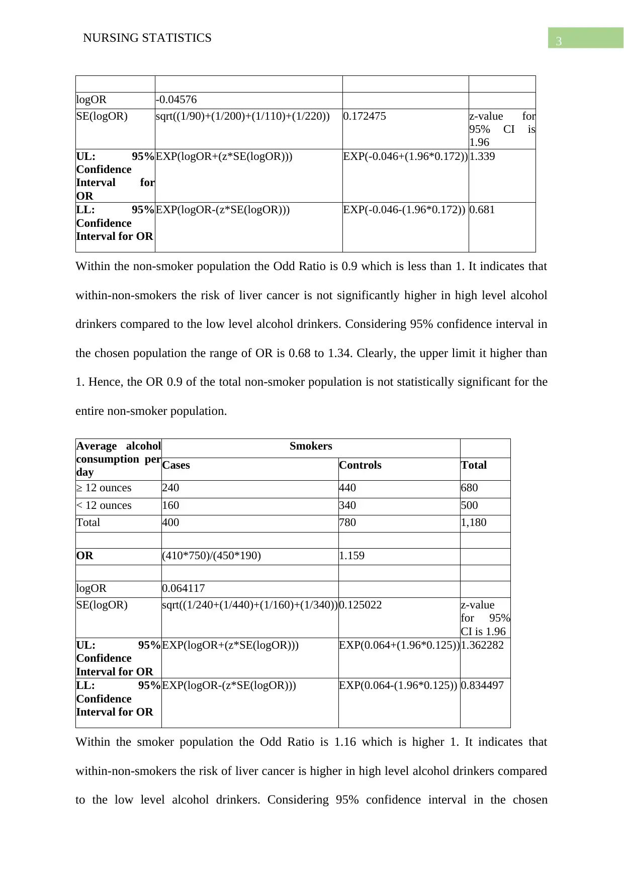
logOR -0.04576
SE(logOR) sqrt((1/90)+(1/200)+(1/110)+(1/220)) 0.172475 z-value for
95% CI is
1.96
UL: 95%
Confidence
Interval for
OR
EXP(logOR+(z*SE(logOR))) EXP(-0.046+(1.96*0.172))1.339
LL: 95%
Confidence
Interval for OR
EXP(logOR-(z*SE(logOR))) EXP(-0.046-(1.96*0.172)) 0.681
Within the non-smoker population the Odd Ratio is 0.9 which is less than 1. It indicates that
within-non-smokers the risk of liver cancer is not significantly higher in high level alcohol
drinkers compared to the low level alcohol drinkers. Considering 95% confidence interval in
the chosen population the range of OR is 0.68 to 1.34. Clearly, the upper limit it higher than
1. Hence, the OR 0.9 of the total non-smoker population is not statistically significant for the
entire non-smoker population.
Average alcohol
consumption per
day
Smokers
Cases Controls Total
≥ 12 ounces 240 440 680
< 12 ounces 160 340 500
Total 400 780 1,180
OR (410*750)/(450*190) 1.159
logOR 0.064117
SE(logOR) sqrt((1/240+(1/440)+(1/160)+(1/340))0.125022 z-value
for 95%
CI is 1.96
UL: 95%
Confidence
Interval for OR
EXP(logOR+(z*SE(logOR))) EXP(0.064+(1.96*0.125))1.362282
LL: 95%
Confidence
Interval for OR
EXP(logOR-(z*SE(logOR))) EXP(0.064-(1.96*0.125)) 0.834497
Within the smoker population the Odd Ratio is 1.16 which is higher 1. It indicates that
within-non-smokers the risk of liver cancer is higher in high level alcohol drinkers compared
to the low level alcohol drinkers. Considering 95% confidence interval in the chosen

4NURSING STATISTICS
population the range of OR is 0.83 to 1.36. Clearly, the upper lower limit is lower than 1.
Hence, the OR 01.16 of the total non-smoker population is not statistically significant for the
entire non-smoker population.
c)
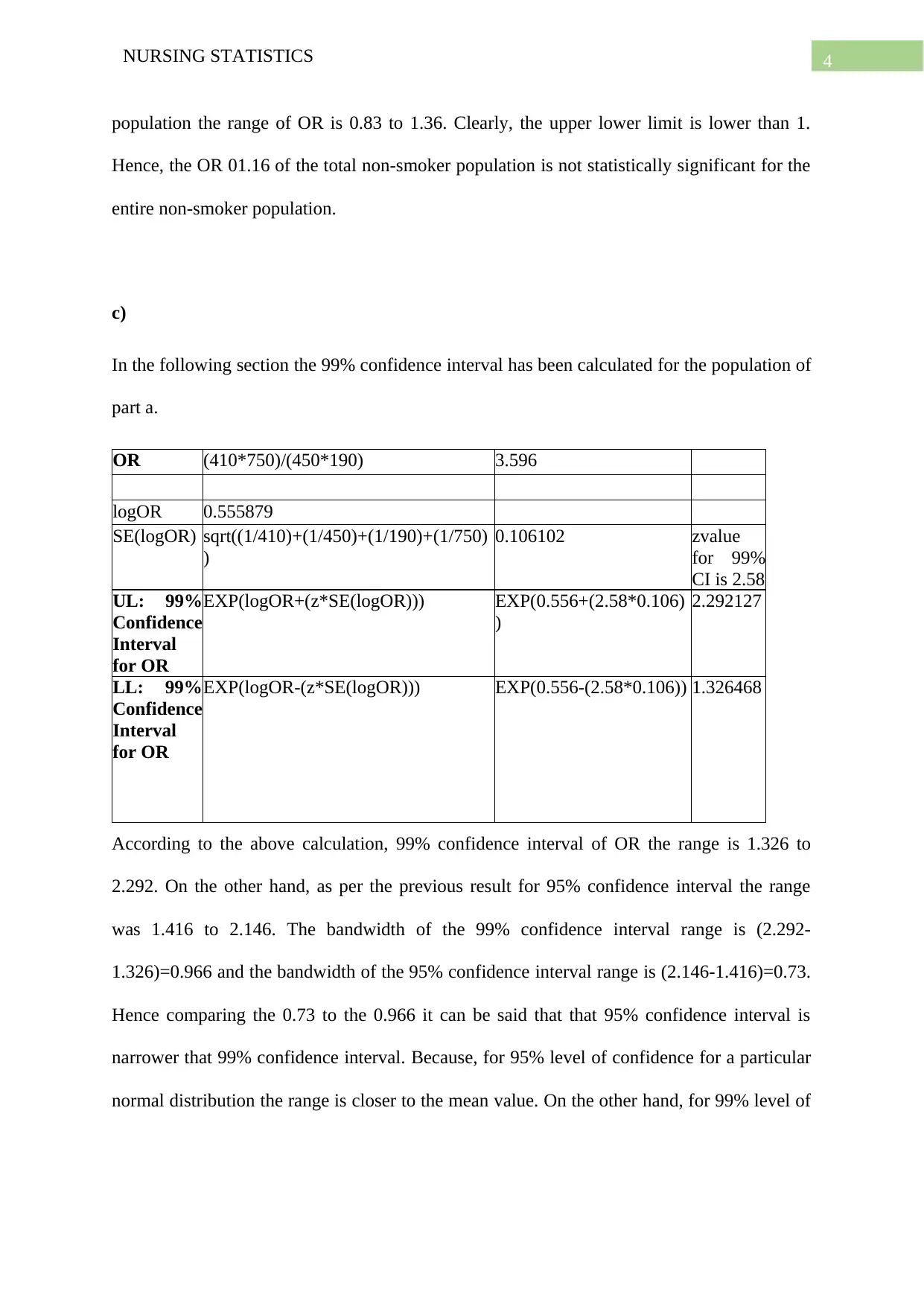
In the following section the 99% confidence interval has been calculated for the population of
part a.
OR (410*750)/(450*190) 3.596
logOR 0.555879
SE(logOR) sqrt((1/410)+(1/450)+(1/190)+(1/750)
)
0.106102 zvalue
for 99%
CI is 2.58
UL: 99%
Confidence
Interval
for OR
EXP(logOR+(z*SE(logOR))) EXP(0.556+(2.58*0.106)
)
2.292127
LL: 99%
Confidence
Interval
for OR
EXP(logOR-(z*SE(logOR))) EXP(0.556-(2.58*0.106)) 1.326468
According to the above calculation, 99% confidence interval of OR the range is 1.326 to
2.292. On the other hand, as per the previous result for 95% confidence interval the range
was 1.416 to 2.146. The bandwidth of the 99% confidence interval range is (2.292-
1.326)=0.966 and the bandwidth of the 95% confidence interval range is (2.146-1.416)=0.73.
Hence comparing the 0.73 to the 0.966 it can be said that that 95% confidence interval is
narrower that 99% confidence interval. Because, for 95% level of confidence for a particular
normal distribution the range is closer to the mean value. On the other hand, for 99% level of

5NURSING STATISTICS
confidence for the same normal distribution the larger section of population had to be
considered and therefore the range shifted away from the mean value.
Question #3
a)
The similarity between prevalence and incidence is that both indicants the level of risk with
same direction. In other words, increment of both prevalence and incidence indicates
increment in risk level.
The major difference between prevalence and incidence is that prevalence refers to the
proportion of population with disease among the total population at risk, whereas incidence
refers to both ratio and rate of occurring new case.
b)
The major similarity between incidence rate and cumulative incidence is that both of these
considers the new cases of disease in their numerator.
The major difference between incidence rate and cumulative incidence is that cumulative
incidents measure the ratio of new case out of total population at risk, whereas incident rate
considers the total amount of time at risk of each and every subjects in its denominator.
Question #4
P value indicates a probability value, which implies the probability of the chosen statistical
statement or findings being wrong. The lower the P-value is the higher accuracy or
significance of the statistical result within the chosen population. As an example if a p value
of statistical result is lower than 0.05, then it is considered significance, otherwise it is
considered insignificant. However, Confidence Interval not only shows the significance of
the statistical result or statement but also the range of probability for being significance. In

6NURSING STATISTICS
case of 95% confidence interval with upper and lower limit of the statistical result, the study
can have better view regarding the results within higher and lower limit of the result
appropriate for 95% and the deviation of the result within rest of the 5% population.
Therefore, Confidence interval provides much more information regarding the statistical
results, its significance and the level of significance in different distribution of the chosen
population.
Question #5
In order to measure the prevalence of cases up to December 31st of 2018, both cases of 2017
and 2018 should be considered where the total population should be taken as per the latest
population of the 2018. Accordingly the following calculations has been done.
Population at risk new Cases of
osteoporosis
Year 2017 70000 4500
Year 2018 70000+10000 2000
Total 80000 6500
prevalenc
e
Cases of osteoporosis/Population at risk 6500/80000 0.08125
Hence assuming none of the osteoporosis cases died, the prevalence of osteoporosis on
December 31, 2018 is (0.08125*100)=8.125%
For cumulative incident of 2018, the new population at risk should be considered excluding
the previous cases in 2017. For cumulative incident only the new cases in 2018 have to be
considered. Accordingly the following calculations has been done.
Population at risk new cases in 2018
Year 2018 total population-cases of year
2017
2000
80000-4500 2000
75500 2000
cumulativ
e
incidence
for 2018
New cases of
osteoporosis/Population at risk
2000/75500 0.02649

7NURSING STATISTICS
The cumulative incidence (risk) of developing osteoporosis among the adult population at
risk during the year 2018 is (0.02649*100)=2.649% or 265 out of 10000 population.
Question #7
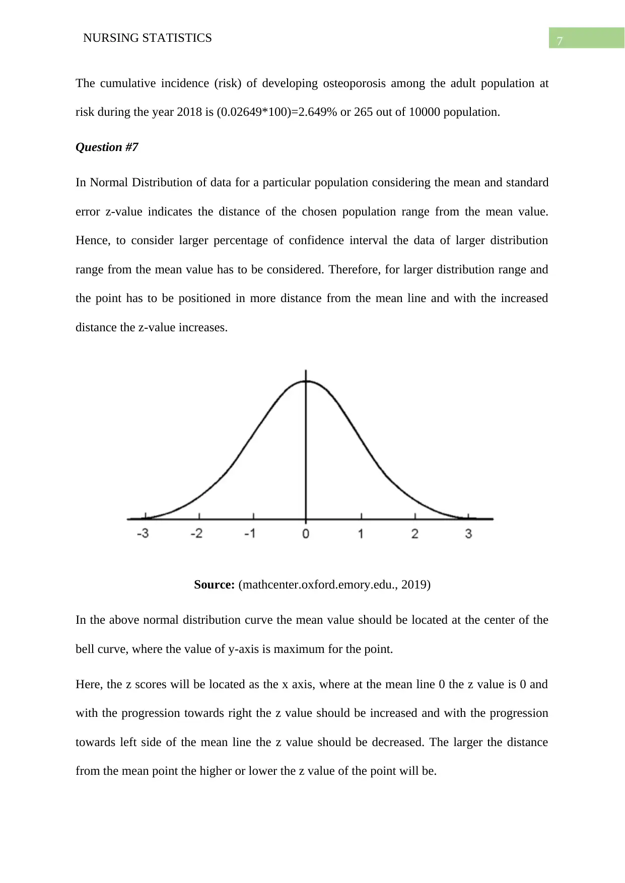
In Normal Distribution of data for a particular population considering the mean and standard
error z-value indicates the distance of the chosen population range from the mean value.
Hence, to consider larger percentage of confidence interval the data of larger distribution
range from the mean value has to be considered. Therefore, for larger distribution range and
the point has to be positioned in more distance from the mean line and with the increased
distance the z-value increases.
Source: (mathcenter.oxford.emory.edu., 2019)
In the above normal distribution curve the mean value should be located at the center of the
bell curve, where the value of y-axis is maximum for the point.
Here, the z scores will be located as the x axis, where at the mean line 0 the z value is 0 and
with the progression towards right the z value should be increased and with the progression
towards left side of the mean line the z value should be decreased. The larger the distance
from the mean point the higher or lower the z value of the point will be.

8NURSING STATISTICS

9NURSING STATISTICS
Bibliography
Collett, D. (2015). Modelling survival data in medical research. Chapman and Hall/CRC.
Greenland, S., Senn, S. J., Rothman, K. J., Carlin, J. B., Poole, C., Goodman, S. N., &
Altman, D. G. (2016). Statistical tests, P values, confidence intervals, and power: a
guide to misinterpretations. European journal of epidemiology, 31(4), 337-350.
mathcenter.oxford.emory.edu. (2019). Retrieved 29 December 2019, from
http://mathcenter.oxford.emory.edu/site/math117/normalDistribution/300-00.gif
Petrie, A., & Sabin, C. (2019). Medical statistics at a glance. John Wiley & Sons.
Stewart, A. (2018). Basic statistics and epidemiology: a practical guide. CRC Press.