Optimisation Problem: Logistics and Supply Chain Management

This article discusses the formulation of multi-objective linear programming for logistics and supply chain management. It includes solutions for reducing transportation costs and finding the location of warehouses. The article also covers the use of the Analytical Hierarchy Process (AHP) to decide the best criteria for Mr. Jones.

Optimisation Problem.
1 | P a g e
Logistics and Supply chain management

Optimisation Problem.
Contents
Solution 1.........................................................................................................................................3
Solution1(a).................................................................................................................................3
Solution1(b).................................................................................................................................6
Solution1(c).................................................................................................................................7
Solution 2.........................................................................................................................................8
2 | P a g e

Optimisation Problem.
Solution 1
Solution1(a)
The formulation of multi objective linear programming start with solving the linear programming
from each variable and combine to make a common objective with and solve this including he
two optimised result obtained from individual objective solving,
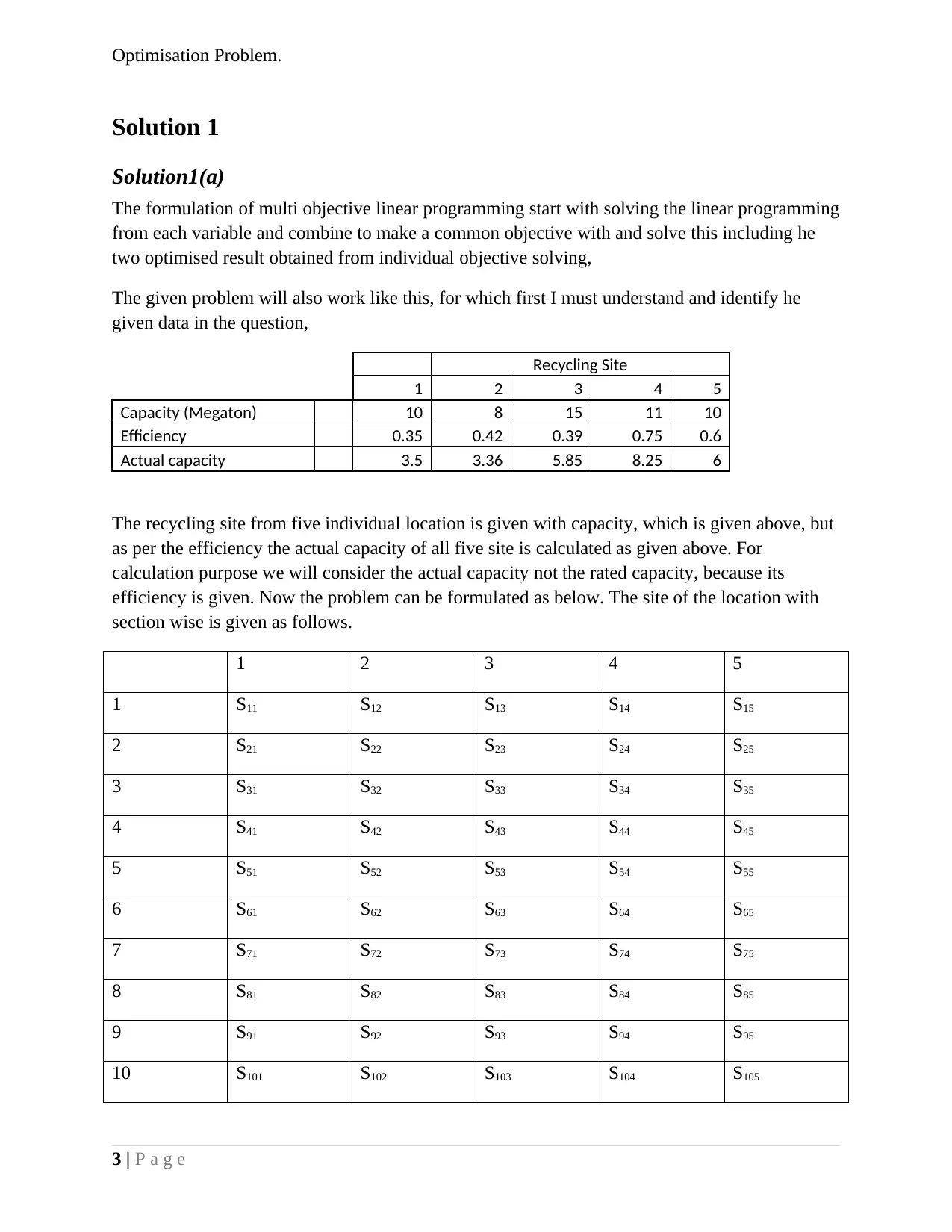
The given problem will also work like this, for which first I must understand and identify he
given data in the question,
Recycling Site
1 2 3 4 5
Capacity (Megaton) 10 8 15 11 10
Efficiency 0.35 0.42 0.39 0.75 0.6
Actual capacity 3.5 3.36 5.85 8.25 6
The recycling site from five individual location is given with capacity, which is given above, but
as per the efficiency the actual capacity of all five site is calculated as given above. For
calculation purpose we will consider the actual capacity not the rated capacity, because its
efficiency is given. Now the problem can be formulated as below. The site of the location with
section wise is given as follows.
1 2 3 4 5
1 S11 S12 S13 S14 S15
2 S21 S22 S23 S24 S25
3 S31 S32 S33 S34 S35
4 S41 S42 S43 S44 S45
5 S51 S52 S53 S54 S55
6 S61 S62 S63 S64 S65
7 S71 S72 S73 S74 S75
8 S81 S82 S83 S84 S85
9 S91 S92 S93 S94 S95
10 S101 S102 S103 S104 S105
3 | P a g e

Optimisation Problem.
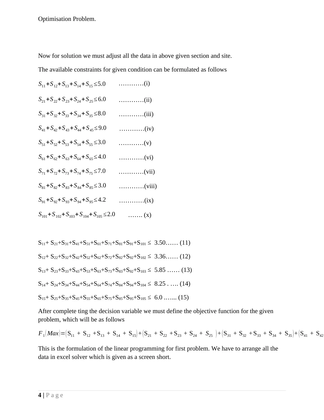
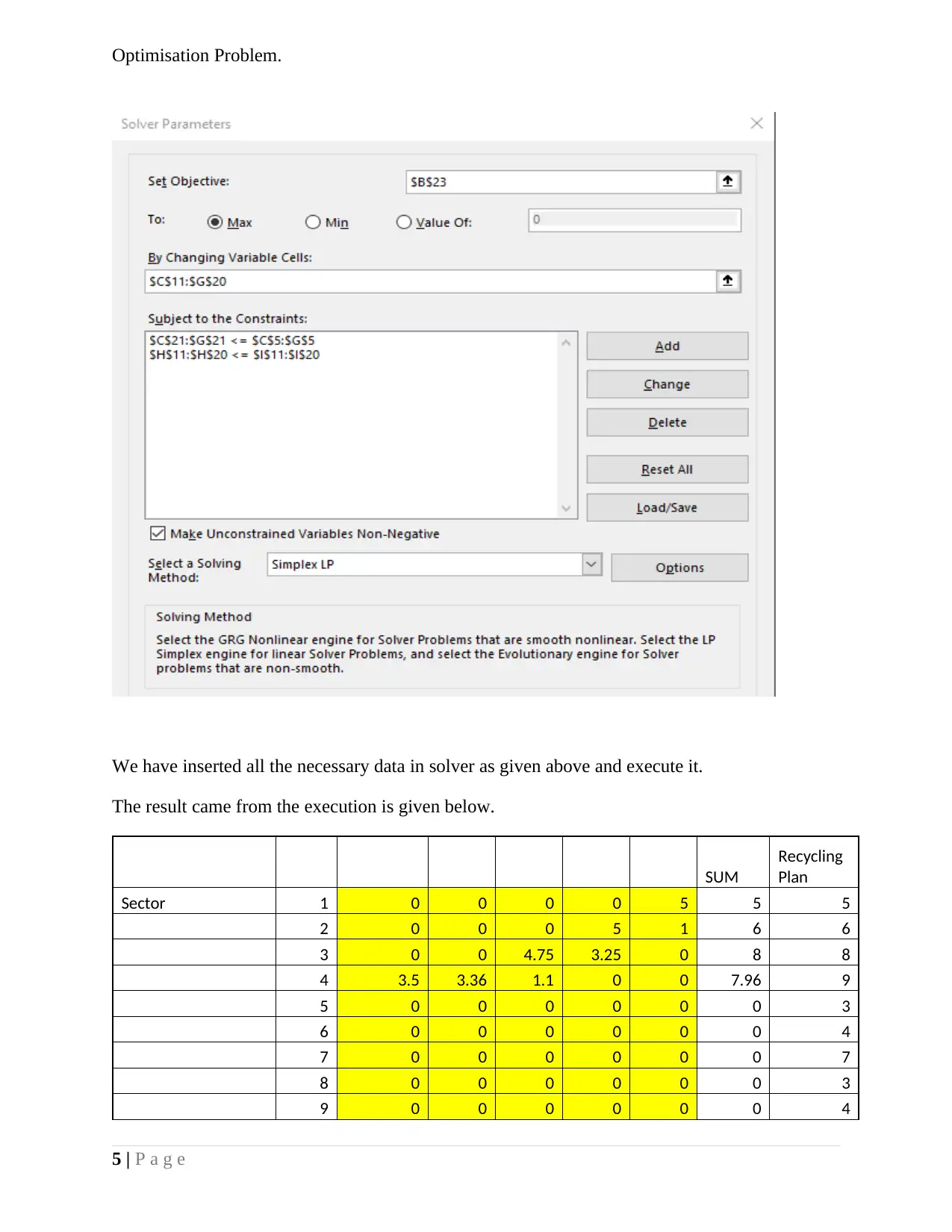
Now for solution we must adjust all the data in above given section and site.
The available constraints for given condition can be formulated as follows
S11 +S12+ S13 + S14 +S15 ≤5.0 …………(i)
S21 +S22+ S23+ S24 +S25 ≤ 6.0 …………(ii)
S31 +S32+S33 +S34 + S35 ≤8.0 …………(iii)
S41 +S42 +S43 + S44 + S45 ≤ 9.0 …………(iv)
S51 +S52+ S53 + S54 +S55 ≤3.0 …………(v)
S61 +S62+ S63+ S64 +S65 ≤ 4.0 …………(vi)
S71 +S72+ S73 + S74 +S75 ≤7.0 …………(vii)
S81 +S82+S83+S84+ S85 ≤ 3.0 …………(viii)
S91 +S92+ S93+ S94 +S95 ≤ 4.2 …………(ix)
S101+S102+ S103+ S104+ S105 ≤2.0 ……. (x)
S11+ S21+S31+S41+S51+S61+S71+S81+S91+S101 ≤ 3.50…… (11)
S12+ S22+S32+S42+S52+S62+S72+S82+S92+S102 ≤ 3.36…… (12)
S13+ S23+S33+S43+S53+S63+S73+S83+S92+S103 ≤ 5.85 …… (13)
S14+ S24+S34+S44+S54+S64+S74+S84+S94+S104 ≤ 8.25 . …. (14)
S15+ S25+S35+S45+S55+S65+S75+S85+S95+S105 ≤ 6.0 .…... (15)
After complete ting the decision variable we must define the objective function for the given
problem, which will be as follows
F1 ( Max ) = ( S11 + S12 +S13 + S14 + S15 ) + ( S21 + S22 + S23 + S24 + S25 ) + ( S31 + S32 + S33 + S34 + S35 ) + ( S41 + S42
This is the formulation of the linear programming for first problem. We have to arrange all the
data in excel solver which is given as a screen short.
4 | P a g e

Optimisation Problem.
We have inserted all the necessary data in solver as given above and execute it.
The result came from the execution is given below.
SUM
Recycling
Plan
Sector 1 0 0 0 0 5 5 5
2 0 0 0 5 1 6 6
3 0 0 4.75 3.25 0 8 8
4 3.5 3.36 1.1 0 0 7.96 9
5 0 0 0 0 0 0 3
6 0 0 0 0 0 0 4
7 0 0 0 0 0 0 7
8 0 0 0 0 0 0 3
9 0 0 0 0 0 0 4
5 | P a g e

Optimisation Problem.
10 0 0 0 0 0 0 2
SUM 3.5 3.36 5.85 8.25 6 26.96 51
Objective function 1 26.96 Maximise
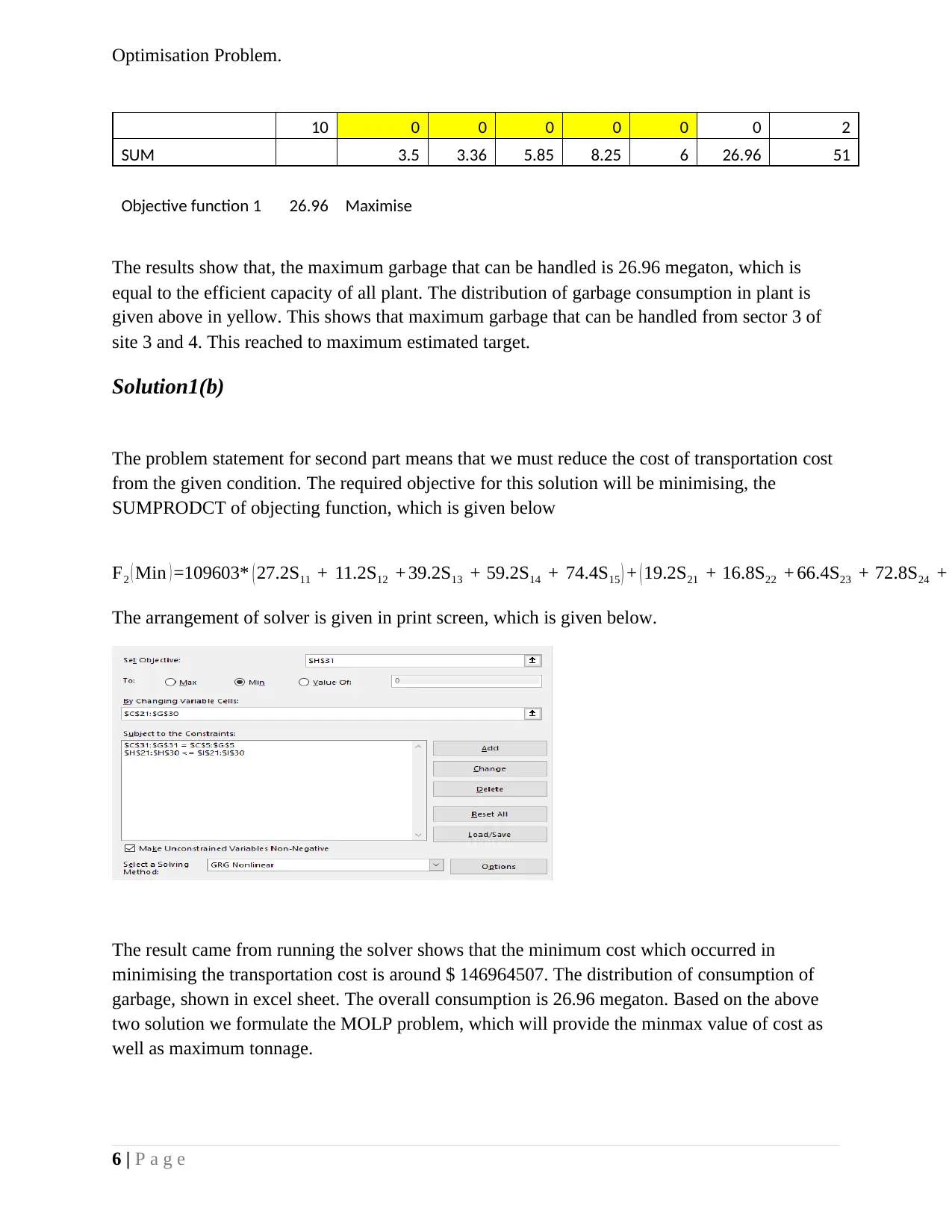
The results show that, the maximum garbage that can be handled is 26.96 megaton, which is
equal to the efficient capacity of all plant. The distribution of garbage consumption in plant is
given above in yellow. This shows that maximum garbage that can be handled from sector 3 of
site 3 and 4. This reached to maximum estimated target.
Solution1(b)
The problem statement for second part means that we must reduce the cost of transportation cost
from the given condition. The required objective for this solution will be minimising, the
SUMPRODCT of objecting function, which is given below
F2 ( Min ) =109603* ( 27.2S11 + 11.2S12 + 39.2S13 + 59.2S14 + 74.4S15 ) + ( 19.2S21 + 16.8S22 + 66.4S23 + 72.8S24 +
The arrangement of solver is given in print screen, which is given below.
The result came from running the solver shows that the minimum cost which occurred in
minimising the transportation cost is around $ 146964507. The distribution of consumption of
garbage, shown in excel sheet. The overall consumption is 26.96 megaton. Based on the above
two solution we formulate the MOLP problem, which will provide the minmax value of cost as
well as maximum tonnage.
6 | P a g e

Optimisation Problem.
Solution1(c)
The multi objective linear programming, dictates the overall optimisation for any problem. At
the given scenario, we have to bring both the solution in same platform, and % deviation is the
tool by which we can do this. Therefore, we must calculate the % deviation and multiply it with
given weight and feed into the solver, which is as follows.
The deviation in % will be calculated as follows.as
M 1= Target tonnage−calculated tonnage
Target tonnage
and M 2= calculated cost−Target cost
Target cost
As given in question, the weightage is triple of cost to the tonnage.
The new constraints will M 1 W 1 ≤ D
M 2 W 2 ≤ D
W 1=3W 2
After feeding the value in the solver, we got the following result.
The minimax value comes around 0, which means that there is no change in MOLP solution, as
it is optimised in the previous state.
Solution 2
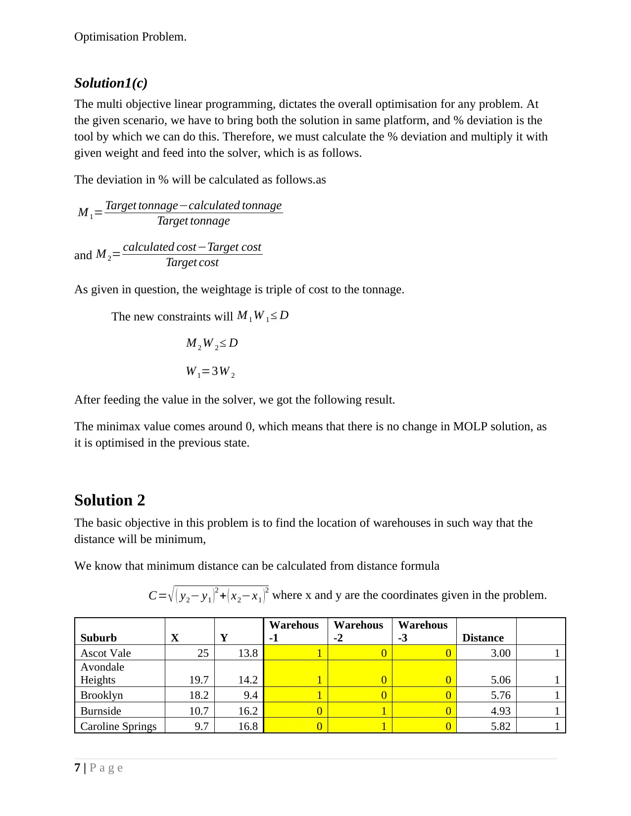
The basic objective in this problem is to find the location of warehouses in such way that the
distance will be minimum,
We know that minimum distance can be calculated from distance formula
C= √ ( y2− y1 ) 2 + ( x2−x1 )
2 where x and y are the coordinates given in the problem.
Suburb X Y
Warehous
-1
Warehous
-2
Warehous
-3 Distance
Ascot Vale 25 13.8 1 0 0 3.00 1
Avondale
Heights 19.7 14.2 1 0 0 5.06 1
Brooklyn 18.2 9.4 1 0 0 5.76 1
Burnside 10.7 16.2 0 1 0 4.93 1
Caroline Springs 9.7 16.8 0 1 0 5.82 1
7 | P a g e

Optimisation Problem.
Derrimut 10.7 10.2 0 1 0 1.71 1
Flemington 24.3 11.8 1 0 0 0.92 1
Footscray 22.4 11 1 0 0 1.30 1
Footscray 23.7 11.1 1 0 0 0.00 1
Hopper Crossing 6.3 4.7 0 0 1 0.94 1
Laverton north 13.5 7.2 0 1 0 4.51 1
Melbourne 28.6 8.9 1 0 0 5.37 1
Seabrook 10.9 2.3 0 0 1 6.12 1
Southbank 29.8 8.1 1 0 0 6.80 1
ST kilda 30.4 3.4 1 0 0 10.21 1
Sunshine west 16.6 10.2 0 1 0 4.86 1
Tarneit 5.2 8.1 0 0 1 3.09 1
tarneit 5.1 6.6 0 0 1 1.62 1
Werribee 0.5 0 0 0 1 7.02 1
Wyndham Vale 0 2 0 0 1 6.20 1
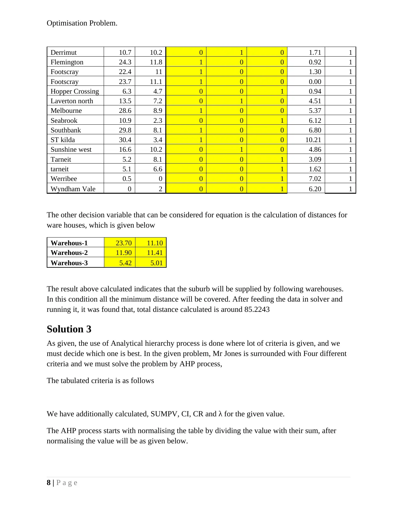
The other decision variable that can be considered for equation is the calculation of distances for
ware houses, which is given below
Warehous-1 23.70 11.10
Warehous-2 11.90 11.41
Warehous-3 5.42 5.01
The result above calculated indicates that the suburb will be supplied by following warehouses.
In this condition all the minimum distance will be covered. After feeding the data in solver and
running it, it was found that, total distance calculated is around 85.2243
Solution 3
As given, the use of Analytical hierarchy process is done where lot of criteria is given, and we
must decide which one is best. In the given problem, Mr Jones is surrounded with Four different
criteria and we must solve the problem by AHP process,
The tabulated criteria is as follows
We have additionally calculated, SUMPV, CI, CR and λ for the given value.
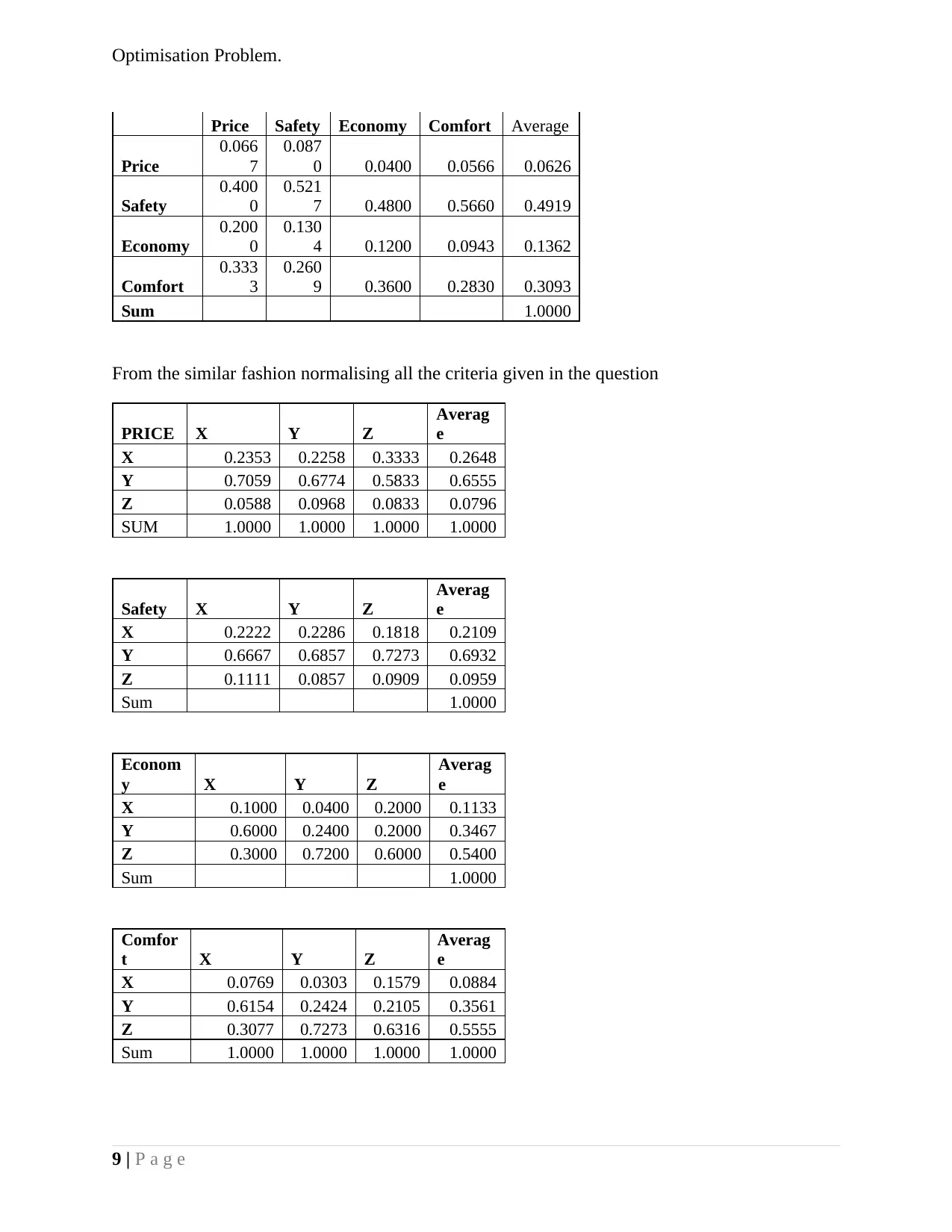
The AHP process starts with normalising the table by dividing the value with their sum, after
normalising the value will be as given below.
8 | P a g e

Optimisation Problem.
Price Safety Economy Comfort Average
Price
0.066
7
0.087
0 0.0400 0.0566 0.0626
Safety
0.400
0
0.521
7 0.4800 0.5660 0.4919
Economy
0.200
0
0.130
4 0.1200 0.0943 0.1362
Comfort
0.333
3
0.260
9 0.3600 0.2830 0.3093
Sum 1.0000
From the similar fashion normalising all the criteria given in the question
PRICE X Y Z
Averag
e
X 0.2353 0.2258 0.3333 0.2648
Y 0.7059 0.6774 0.5833 0.6555
Z 0.0588 0.0968 0.0833 0.0796
SUM 1.0000 1.0000 1.0000 1.0000
Safety X Y Z
Averag
e
X 0.2222 0.2286 0.1818 0.2109
Y 0.6667 0.6857 0.7273 0.6932
Z 0.1111 0.0857 0.0909 0.0959
Sum 1.0000
Econom
y X Y Z
Averag
e
X 0.1000 0.0400 0.2000 0.1133
Y 0.6000 0.2400 0.2000 0.3467
Z 0.3000 0.7200 0.6000 0.5400
Sum 1.0000
Comfor
t X Y Z
Averag
e
X 0.0769 0.0303 0.1579 0.0884
Y 0.6154 0.2424 0.2105 0.3561
Z 0.3077 0.7273 0.6316 0.5555
Sum 1.0000 1.0000 1.0000 1.0000
9 | P a g e

Optimisation Problem.
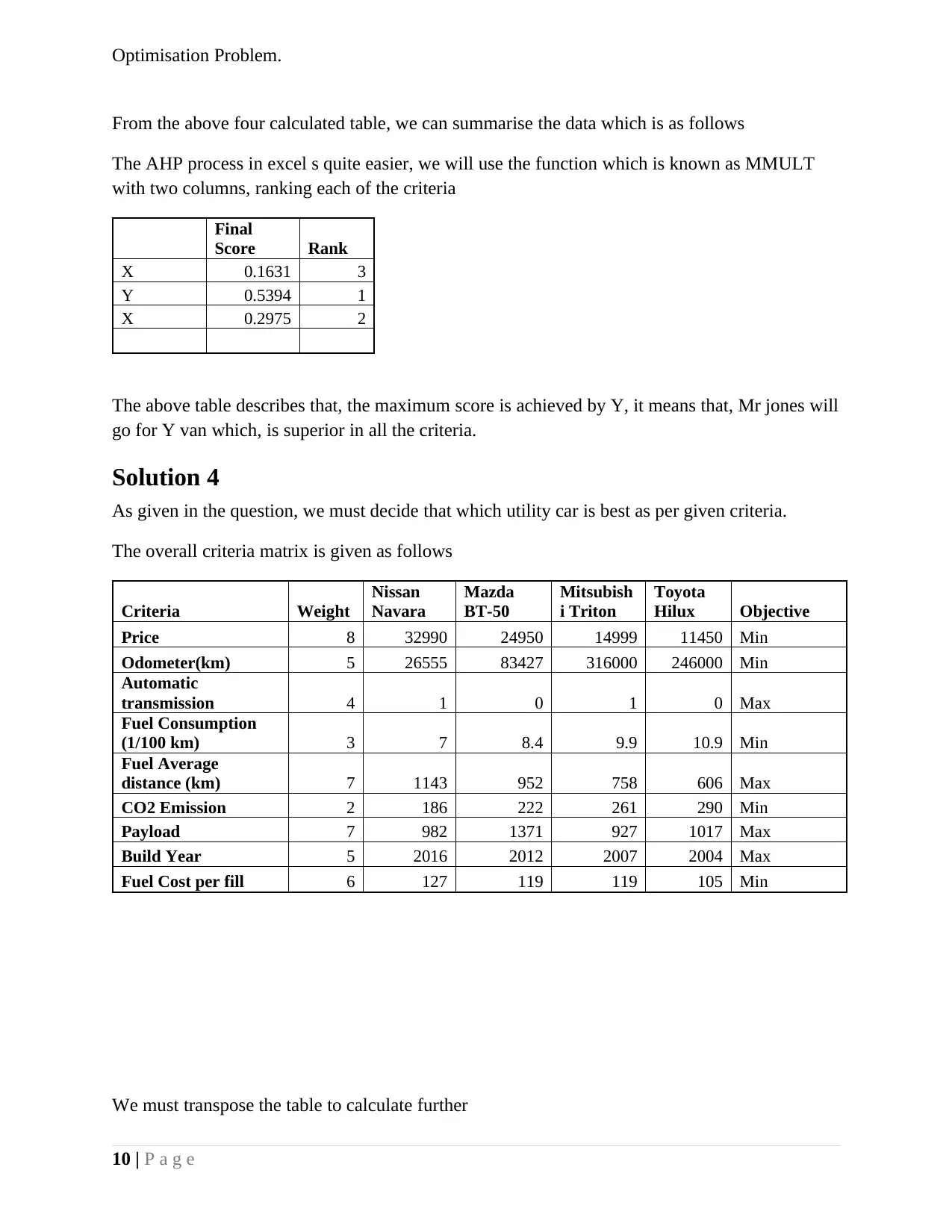
From the above four calculated table, we can summarise the data which is as follows
The AHP process in excel s quite easier, we will use the function which is known as MMULT
with two columns, ranking each of the criteria
Final
Score Rank
X 0.1631 3
Y 0.5394 1
X 0.2975 2
The above table describes that, the maximum score is achieved by Y, it means that, Mr jones will
go for Y van which, is superior in all the criteria.
Solution 4
As given in the question, we must decide that which utility car is best as per given criteria.
The overall criteria matrix is given as follows
Criteria Weight
Nissan
Navara
Mazda
BT-50
Mitsubish
i Triton
Toyota
Hilux Objective
Price 8 32990 24950 14999 11450 Min
Odometer(km) 5 26555 83427 316000 246000 Min
Automatic
transmission 4 1 0 1 0 Max
Fuel Consumption
(1/100 km) 3 7 8.4 9.9 10.9 Min
Fuel Average
distance (km) 7 1143 952 758 606 Max
CO2 Emission 2 186 222 261 290 Min
Payload 7 982 1371 927 1017 Max
Build Year 5 2016 2012 2007 2004 Max
Fuel Cost per fill 6 127 119 119 105 Min
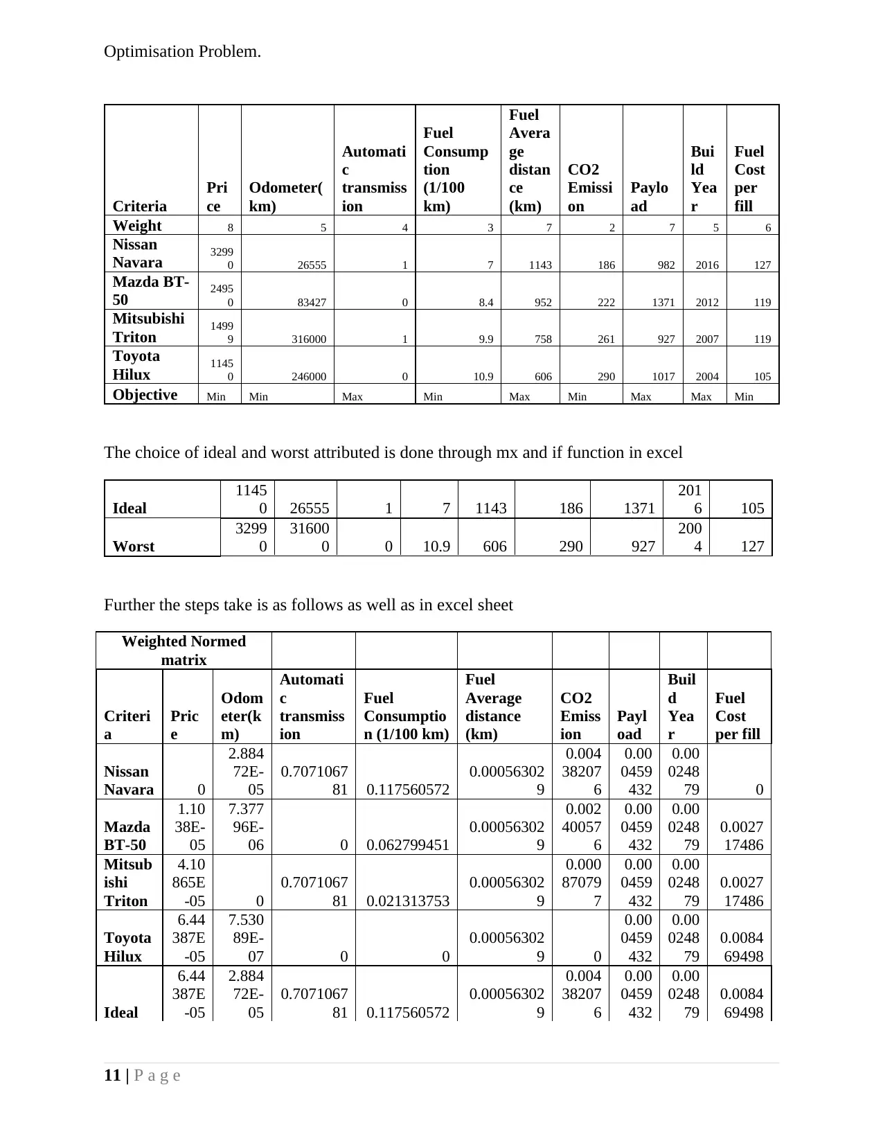
We must transpose the table to calculate further
10 | P a g e

Optimisation Problem.
Criteria
Pri
ce
Odometer(
km)
Automati
c
transmiss
ion
Fuel
Consump
tion
(1/100
km)
Fuel
Avera
ge
distan
ce
(km)
CO2
Emissi
on
Paylo
ad
Bui
ld
Yea
r
Fuel
Cost
per
fill
Weight 8 5 4 3 7 2 7 5 6
Nissan
Navara 3299
0 26555 1 7 1143 186 982 2016 127
Mazda BT-
50 2495
0 83427 0 8.4 952 222 1371 2012 119
Mitsubishi
Triton 1499
9 316000 1 9.9 758 261 927 2007 119
Toyota
Hilux 1145
0 246000 0 10.9 606 290 1017 2004 105
Objective Min Min Max Min Max Min Max Max Min
The choice of ideal and worst attributed is done through mx and if function in excel
Ideal
1145
0 26555 1 7 1143 186 1371
201
6 105
Worst
3299
0
31600
0 0 10.9 606 290 927
200
4 127
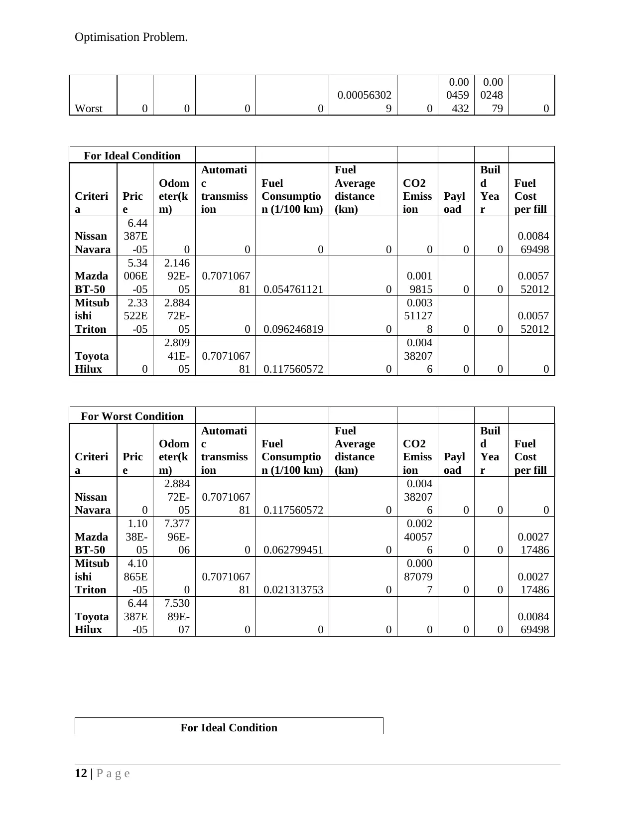
Further the steps take is as follows as well as in excel sheet
Weighted Normed
matrix
Criteri
a
Pric
e
Odom
eter(k
m)
Automati
c
transmiss
ion
Fuel
Consumptio
n (1/100 km)
Fuel
Average
distance
(km)
CO2
Emiss
ion
Payl
oad
Buil
d
Yea
r
Fuel
Cost
per fill
Nissan
Navara 0
2.884
72E-
05
0.7071067
81 0.117560572
0.00056302
9
0.004
38207
6
0.00
0459
432
0.00
0248
79 0
Mazda
BT-50
1.10
38E-
05
7.377
96E-
06 0 0.062799451
0.00056302
9
0.002
40057
6
0.00
0459
432
0.00
0248
79
0.0027
17486
Mitsub
ishi
Triton
4.10
865E
-05 0
0.7071067
81 0.021313753
0.00056302
9
0.000
87079
7
0.00
0459
432
0.00
0248
79
0.0027
17486
Toyota
Hilux
6.44
387E
-05
7.530
89E-
07 0 0
0.00056302
9 0
0.00
0459
432
0.00
0248
79
0.0084
69498
Ideal
6.44
387E
-05
2.884
72E-
05
0.7071067
81 0.117560572
0.00056302
9
0.004
38207
6
0.00
0459
432
0.00
0248
79
0.0084
69498
11 | P a g e

Optimisation Problem.
Worst 0 0 0 0
0.00056302
9 0
0.00
0459
432
0.00
0248
79 0
For Ideal Condition
Criteri
a
Pric
e
Odom
eter(k
m)
Automati
c
transmiss
ion
Fuel
Consumptio
n (1/100 km)
Fuel
Average
distance
(km)
CO2
Emiss
ion
Payl
oad
Buil
d
Yea
r
Fuel
Cost
per fill
Nissan
Navara
6.44
387E
-05 0 0 0 0 0 0 0
0.0084
69498
Mazda
BT-50
5.34
006E
-05
2.146
92E-
05
0.7071067
81 0.054761121 0
0.001
9815 0 0
0.0057
52012
Mitsub
ishi
Triton
2.33
522E
-05
2.884
72E-
05 0 0.096246819 0
0.003
51127
8 0 0
0.0057
52012
Toyota
Hilux 0
2.809
41E-
05
0.7071067
81 0.117560572 0
0.004
38207
6 0 0 0
For Worst Condition
Criteri
a
Pric
e
Odom
eter(k
m)
Automati
c
transmiss
ion
Fuel
Consumptio
n (1/100 km)
Fuel
Average
distance
(km)
CO2
Emiss
ion
Payl
oad
Buil
d
Yea
r
Fuel
Cost
per fill
Nissan
Navara 0
2.884
72E-
05
0.7071067
81 0.117560572 0
0.004
38207
6 0 0 0
Mazda
BT-50
1.10
38E-
05
7.377
96E-
06 0 0.062799451 0
0.002
40057
6 0 0
0.0027
17486
Mitsub
ishi
Triton
4.10
865E
-05 0
0.7071067
81 0.021313753 0
0.000
87079
7 0 0
0.0027
17486
Toyota
Hilux
6.44
387E
-05
7.530
89E-
07 0 0 0 0 0 0
0.0084
69498
For Ideal Condition
12 | P a g e

Optimisation Problem.
Criteria Value RANK
Nissan Navara 0.008469743 4
Mazda BT-50 0.709250164 2
Mitsubishi Triton 0.096482466 3
Toyota Hilux 0.716826124 1
For Worst Condition
Criteria Value RANK
Nissan Navara 0.716826124 1
Mazda BT-50 0.062904044 3
Mitsubishi Triton 0.707433686 2
Toyota Hilux 0.008469743 4
From Ideal and worst condition ranking for Ideal and worst condition is maximum for Toyota
Hilux. Therefore, the trader must select Toyota Hilux.
13 | P a g e

Optimisation Problem.
References
Bolumole, K, L, 2009, The Customer Service Management Process, The International Journal of
Logistics Management, 14(2), pp, 1-33.
David, Z,, Gilbert , N, N, & Gary, Y, 2016, Supply chain risk management and hospital
inventory: Effects of system affiliation, Journal of Operations Management, 44(1), pp, 30-47.
Gomes, R, 2011, Physical Distribution Service, Jams, 1(1), pp, 1-10.
Gulc, A,, 2017, Models and Methods of Measuring the Quality of Logistic Service, Project, and
Production Management, 255(264), pp, 1-10.
14 | P a g e