Linearization and Performance Optimization of Tricycle Mobile Robots

The study focuses on the kinematic modeling and design analysis of a tricycle mobile robot system, crucial for achieving effective autonomous navigation in robotics applications. Using MATLAB software, this paper simulates and analyzes the kinematics of three-wheeled robots to ensure precision in trajectory control and movement planning. The research identifies key assumptions such as level ground operation and evaluates variations observed during simulations. A linearized model is derived from experimental data to enhance performance, offering a range of motion that adheres closely to real-world dynamics. Ultimately, the paper suggests further exploration into intelligent autonomous systems, focusing on navigation challenges like self-localization, trajectory tracking, and obstacle avoidance. It concludes with recommendations for ongoing research in mobile robotics, emphasizing task planning and sensor integration.

UNIVERSITY AFFILIATION
COURSE NAME & COURSE CODE
DATE OF SUBMISSION
GROUP 5
GROUP REPORT
STUDENT NAME(S) REGISTRATION NUMBER
(S)
% CONTRIBUTION OF
WORK

EXECUTIVE SUMMARY
The paper seeks to derive the kinematic modelling equations in two states where the front wheel
does the steering and the rear wheel roll over and where the front wheels do both the steering and
driving. It, further, seeks to review the concept of wheeled mobile robotics using the tricycle.
The tricycle is a three-wheeled vehicle that is able to move forward and back but it encounters a
lateral slip when it moves sideways. The tricycle, in a practical circumstance, encounters the
ground dynamics and hindrances such as friction. The simulation demonstrates different driving
modes such as constant driving velocity and a constant steering angle, constant driving velocity
and a linearly changing steering angle, and the linearly changing driving velocity with linearly
changing steering angle. The movement of a tricycle is only restricted to forward and backward
movement as opposed to other multi-directional vehicles that can move even sideways
(Giovanni, 2009).
1

TABLE OF CONTENTS
EXECUTIVE SUMMARY.........................................................................................................................1
INTRODUCTION.......................................................................................................................................3
MATLAB IMPLEMENTATION OF THE TRICYCLE.............................................................................6
PART 1....................................................................................................................................................6
PART 2..................................................................................................................................................24
REVIEW AND DISCUSSION..................................................................................................................28
CONCLUSION.........................................................................................................................................30
RECOMMENDATION.............................................................................................................................30
REFERENCES..........................................................................................................................................31
2

INTRODUCTION
The kinematic model of the wheeled mobile robot provides all the feasible directions for the
instantaneous motion. It describes the relation between the velocity input commands and the
derivatives of generalized coordinates (Dong-Sung, & et al., 2003). It is crucial to note that the
highest number of robot locomotives are based on the differential drive model. The model states
that the two powered wheels are used to drive the robot as well as change its direction, hence
they are used for both driving and steering. The control strategies for the differential drive model
of the robot are completely different and do not apply to other robot designs such as the
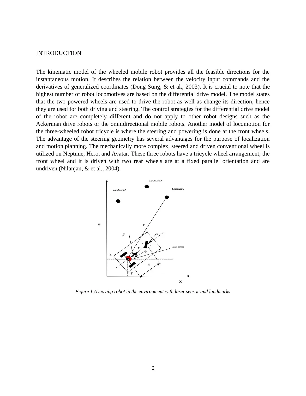
Ackerman drive robots or the omnidirectional mobile robots. Another model of locomotion for
the three-wheeled robot tricycle is where the steering and powering is done at the front wheels.
The advantage of the steering geometry has several advantages for the purpose of localization
and motion planning. The mechanically more complex, steered and driven conventional wheel is
utilized on Neptune, Hero, and Avatar. These three robots have a tricycle wheel arrangement; the
front wheel and it is driven with two rear wheels are at a fixed parallel orientation and are
undriven (Nilanjan, & et al., 2004).
Figure 1 A moving robot in the environment with laser sensor and landmarks
3

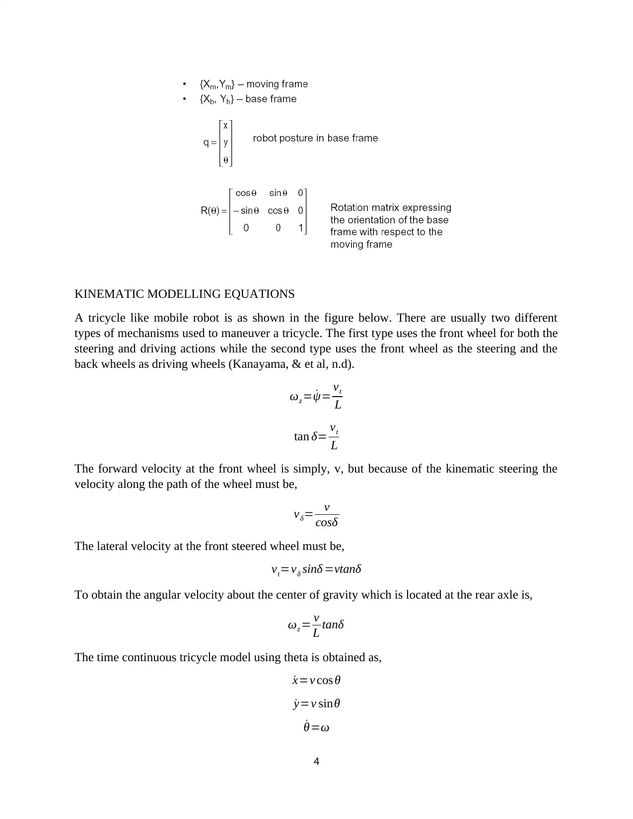
KINEMATIC MODELLING EQUATIONS
A tricycle like mobile robot is as shown in the figure below. There are usually two different
types of mechanisms used to maneuver a tricycle. The first type uses the front wheel for both the
steering and driving actions while the second type uses the front wheel as the steering and the
back wheels as driving wheels (Kanayama, & et al, n.d).
ωz = ˙ψ= vt
L
tan δ= vt
L
The forward velocity at the front wheel is simply, v, but because of the kinematic steering the
velocity along the path of the wheel must be,
vδ= v
cosδ
The lateral velocity at the front steered wheel must be,
vt=vδ sinδ =vtanδ
To obtain the angular velocity about the center of gravity which is located at the rear axle is,
ωz = v
L tanδ
The time continuous tricycle model using theta is obtained as,
˙x=v cosθ
˙y=v sinθ
˙θ=ω
4

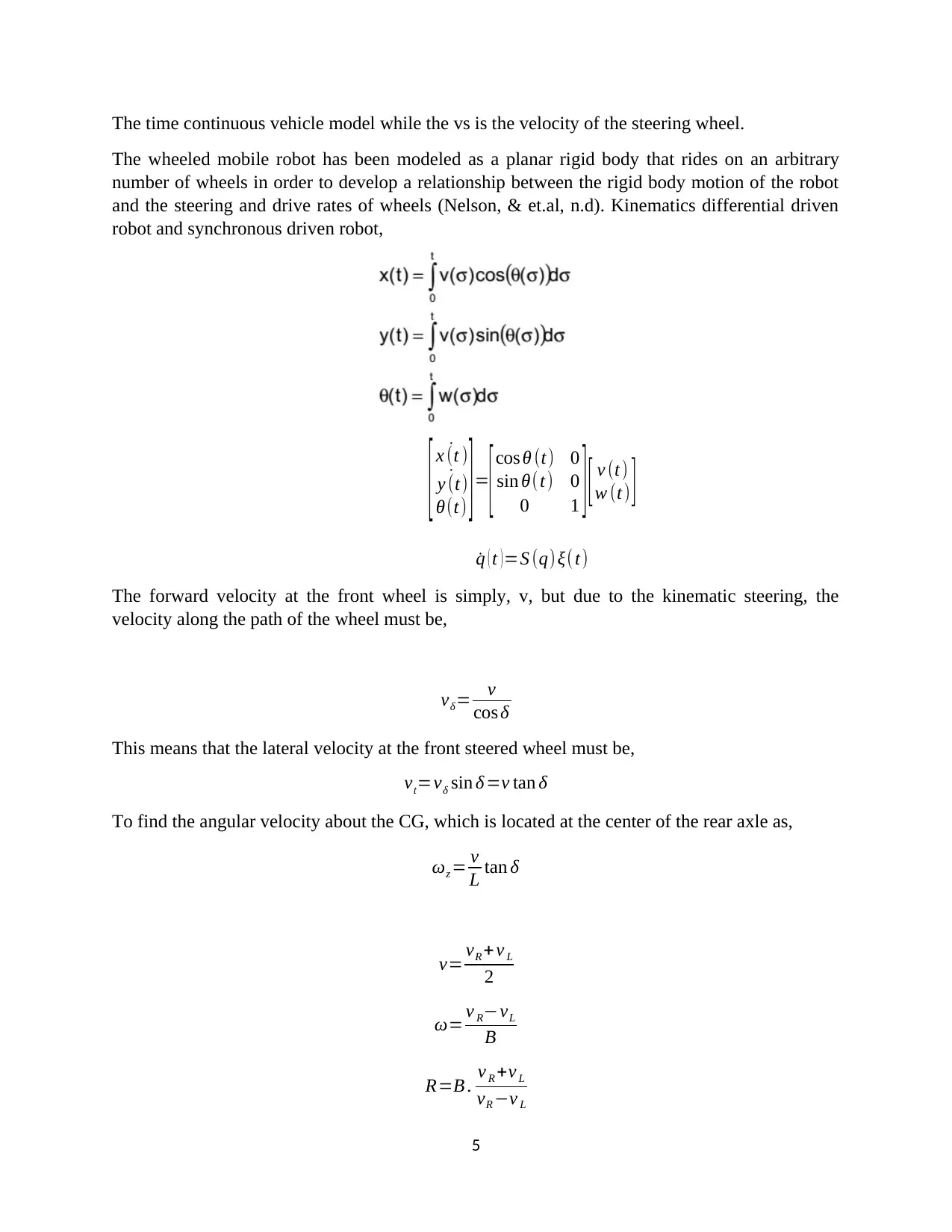
The time continuous vehicle model while the vs is the velocity of the steering wheel.
The wheeled mobile robot has been modeled as a planar rigid body that rides on an arbitrary
number of wheels in order to develop a relationship between the rigid body motion of the robot
and the steering and drive rates of wheels (Nelson, & et.al, n.d). Kinematics differential driven
robot and synchronous driven robot,
[ ˙x (t )
˙y (t)
θ(t) ] =
[ cos θ (t) 0
sin θ(t) 0
0 1 ] [ v (t)
w (t) ]
˙q ( t ) =S (q) ξ(t)
The forward velocity at the front wheel is simply, v, but due to the kinematic steering, the
velocity along the path of the wheel must be,
vδ= v
cos δ
This means that the lateral velocity at the front steered wheel must be,
vt=vδ sin δ =v tan δ
To find the angular velocity about the CG, which is located at the center of the rear axle as,
ωz = v
L tan δ
v= vR + v L
2
ω= v R−vL
B
R=B . v R +v L
vR −v L
5

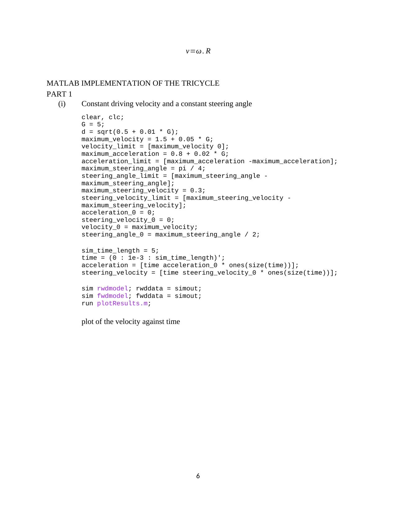
v=ω . R
MATLAB IMPLEMENTATION OF THE TRICYCLE
PART 1
(i) Constant driving velocity and a constant steering angle
clear, clc;
G = 5;
d = sqrt(0.5 + 0.01 * G);
maximum_velocity = 1.5 + 0.05 * G;
velocity_limit = [maximum_velocity 0];
maximum_acceleration = 0.8 + 0.02 * G;
acceleration_limit = [maximum_acceleration -maximum_acceleration];
maximum_steering_angle = pi / 4;
steering_angle_limit = [maximum_steering_angle -
maximum_steering_angle];
maximum_steering_velocity = 0.3;
steering_velocity_limit = [maximum_steering_velocity -
maximum_steering_velocity];
acceleration_0 = 0;
steering_velocity_0 = 0;
velocity_0 = maximum_velocity;
steering_angle_0 = maximum_steering_angle / 2;
sim_time_length = 5;
time = (0 : 1e-3 : sim_time_length)';
acceleration = [time acceleration_0 * ones(size(time))];
steering_velocity = [time steering_velocity_0 * ones(size(time))];
sim rwdmodel; rwddata = simout;
sim fwdmodel; fwddata = simout;
run plotResults.m;
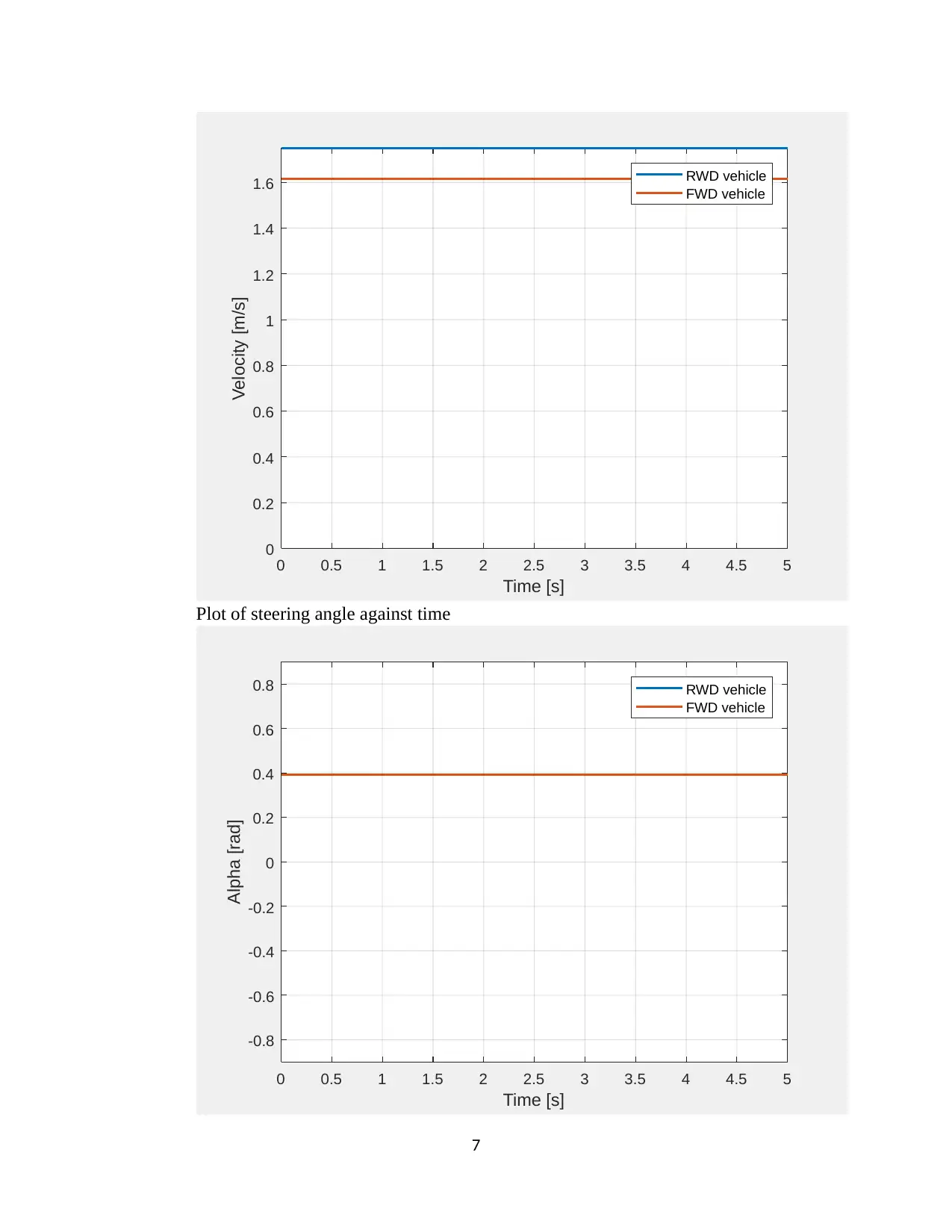
plot of the velocity against time
6

0 0.5 1 1.5 2 2.5 3 3.5 4 4.5 5
Time [s]
0
0.2
0.4
0.6
0.8
1
1.2
1.4
1.6
Velocity [m/s]
RWD vehicle
FWD vehicle
Plot of steering angle against time
0 0.5 1 1.5 2 2.5 3 3.5 4 4.5 5
Time [s]
-0.8
-0.6
-0.4
-0.2
0
0.2
0.4
0.6
0.8
Alpha [rad]
RWD vehicle
FWD vehicle
7

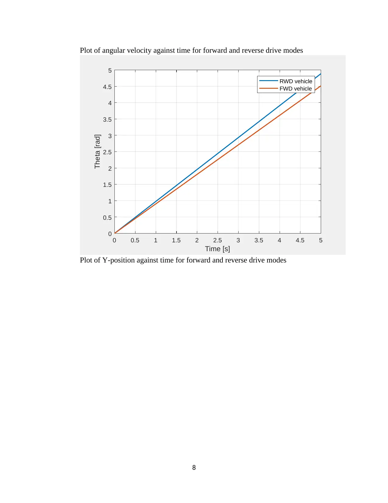
Plot of angular velocity against time for forward and reverse drive modes
0 0.5 1 1.5 2 2.5 3 3.5 4 4.5 5
Time [s]
0
0.5
1
1.5
2
2.5
3
3.5
4
4.5
5
Theta [rad]
RWD vehicle
FWD vehicle
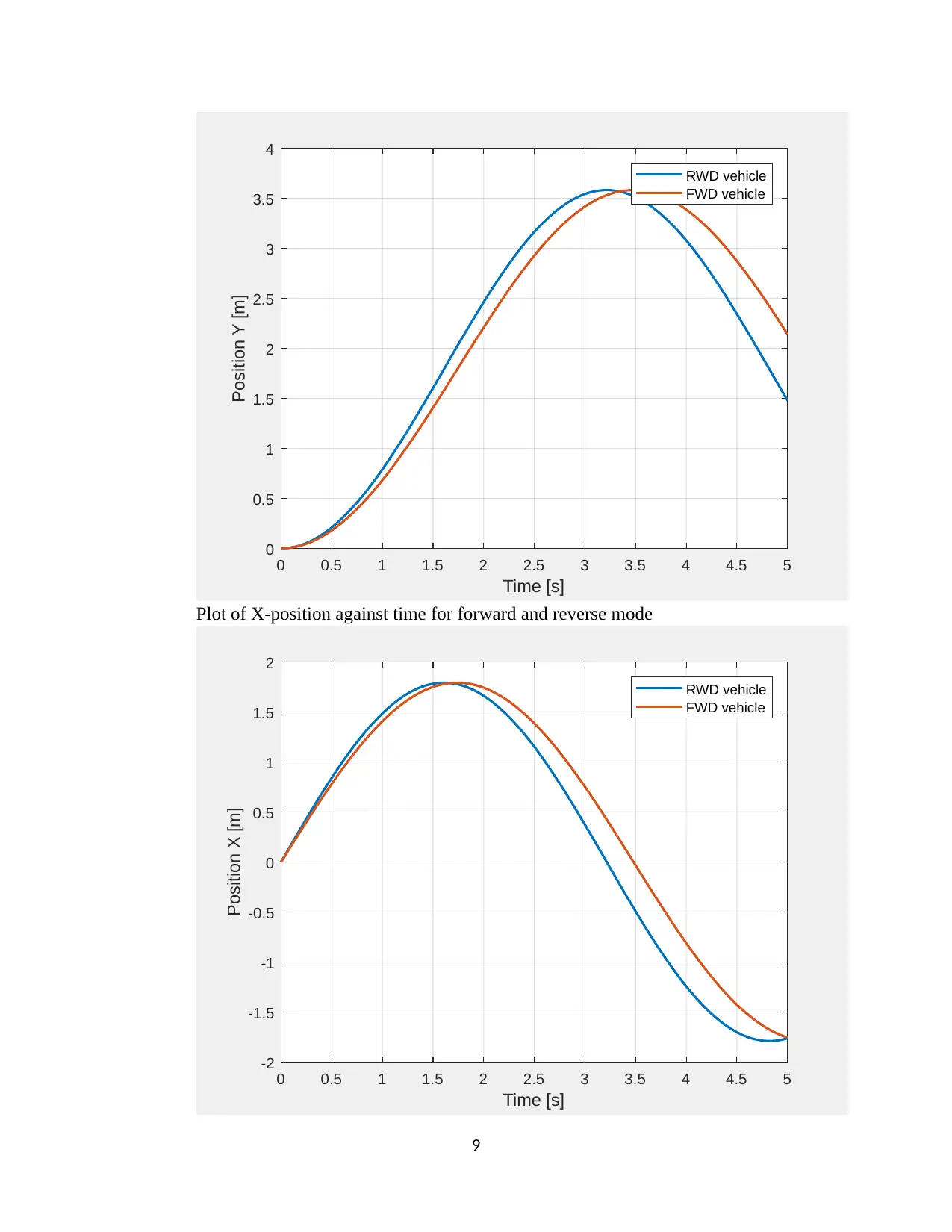
Plot of Y-position against time for forward and reverse drive modes
8

0 0.5 1 1.5 2 2.5 3 3.5 4 4.5 5
Time [s]
0
0.5
1
1.5
2
2.5
3
3.5
4
Position Y [m]
RWD vehicle
FWD vehicle
Plot of X-position against time for forward and reverse mode
0 0.5 1 1.5 2 2.5 3 3.5 4 4.5 5
Time [s]
-2
-1.5
-1
-0.5
0
0.5
1
1.5
2
Position X [m]
RWD vehicle
FWD vehicle
9

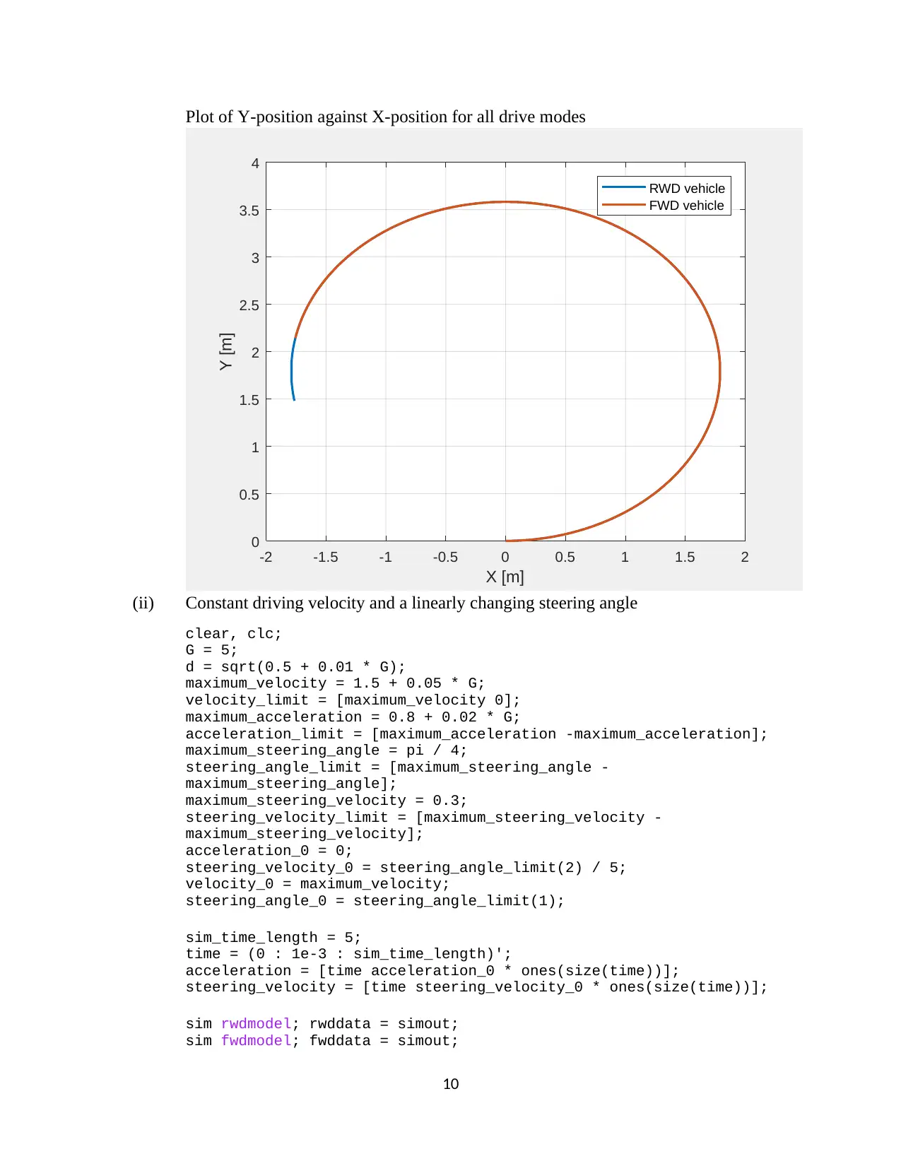
Plot of Y-position against X-position for all drive modes
-2 -1.5 -1 -0.5 0 0.5 1 1.5 2
X [m]
0
0.5
1
1.5
2
2.5
3
3.5
4
Y [m]
RWD vehicle
FWD vehicle
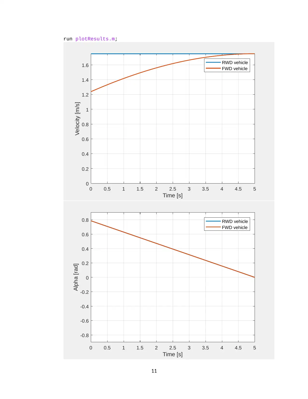
(ii) Constant driving velocity and a linearly changing steering angle
clear, clc;
G = 5;
d = sqrt(0.5 + 0.01 * G);
maximum_velocity = 1.5 + 0.05 * G;
velocity_limit = [maximum_velocity 0];
maximum_acceleration = 0.8 + 0.02 * G;
acceleration_limit = [maximum_acceleration -maximum_acceleration];
maximum_steering_angle = pi / 4;
steering_angle_limit = [maximum_steering_angle -
maximum_steering_angle];
maximum_steering_velocity = 0.3;
steering_velocity_limit = [maximum_steering_velocity -
maximum_steering_velocity];
acceleration_0 = 0;
steering_velocity_0 = steering_angle_limit(2) / 5;
velocity_0 = maximum_velocity;
steering_angle_0 = steering_angle_limit(1);
sim_time_length = 5;
time = (0 : 1e-3 : sim_time_length)';
acceleration = [time acceleration_0 * ones(size(time))];
steering_velocity = [time steering_velocity_0 * ones(size(time))];
sim rwdmodel; rwddata = simout;
sim fwdmodel; fwddata = simout;
10

run plotResults.m;
0 0.5 1 1.5 2 2.5 3 3.5 4 4.5 5
Time [s]
0
0.2
0.4
0.6
0.8
1
1.2
1.4
1.6
Velocity [m/s]
RWD vehicle
FWD vehicle
0 0.5 1 1.5 2 2.5 3 3.5 4 4.5 5
Time [s]
-0.8
-0.6
-0.4
-0.2
0
0.2
0.4
0.6
0.8
Alpha [rad]
RWD vehicle
FWD vehicle
11