Diabetes Prediction Using R

This R assignment delves into the analysis of a diabetes dataset. Students will perform exploratory data analysis using visualizations like boxplots to understand relationships between various variables (e.g., glucose levels, blood pressure) and the outcome (diabetes presence). The core of the assignment involves developing logistic regression models to predict diabetes based on these factors. Model performance is evaluated, and potentially less significant variables are removed to improve model efficiency. Hypothesis testing using t-tests and chi-square tests will be conducted to assess statistical differences between diabetic and non-diabetic groups for key variables.

Women and Diabetes
WOMEN AND DIABETES
Author: ________________

Women and Diabetes
Abstract
This paper focus to test hypotheses revolving around the development of diabetes for women based on
several diagnostic among other factors such as the number of pregnancies and pedigree function. Also, a
logistic regression model is developed to predict the probability of developing diabetes based on several
factors included in the model.
Keyword: BMI – Body Mass Index, GLM –Generalized Linear Models, CatBMI – Categorical variable for BMI <
30 and ≤30
1. INTRODUCTION
Diabetes is a condition caused by increased levels of blood glucose and can be prevented and
managed effectively when diagnosed [1] [2]. The elevated blood glucose levels in the body
increase the risk of having several health conditions such as; nerve damage, kidney problems, heart
diseases and eye problems among others. According to health surveillance statistics in 2014,
around 9.3% of U.S citizens who are aged above 20 years have diabetes [3]. Despite the high
prevalence of the condition, close to 25% of the disease does not know about their status. The
health department has raised concerns for the need of diagnostic tests for the population under risk
of being diabetic to enable them to engage in preventive and management measures. Controlled
diabetes reduces the risk of developing the health conditions mentioned above. Therefore, it is very
important to sensitize people to undertake the required diagnostic measures to monitor their sugar
levels over time.
There are two types of diabetes which include; type 1 and type 2. Type I diabetes is
characterized by the body’s immune system destroying the cells responsible for insulin production.
In this case, insufficient production of insulin leads to reduced sugar absorption in the body. The
patients end up feeling weak because glucose is required for energy production. On the other hand,
type 2 diabetes patients’ body is not able to utilize insulin in the right manner, hence resulting in
the same issues as type 1. Therefore, individuals suffering from type 1 diabetes will show
indications of low blood sugars while those with type 2 diabetes will show high levels. Also,
pregnant women are at risk of developing gestational diabetes which can only be tested 24 and 28th
weeks of pregnancy. There is a chance that the patient will develop type 2 diabetes after giving
birth. This paper will focus on prediction on whether a woman above 21 years will develop
diabetes based on some diagnostic measures. The variables to be considered include the number of
times an individual has been pregnant, glucose levels, diastolic blood pressure, insulin, BMI, skin
thickness, age and diabetes pedigree function.
1.1 Research Questions
i. What is nature statistical relationships between the outcome variable [being diabetic] and
the independent variables?
ii. What is the set of predictor variables, which provide maximum evidence in connection to
the outcome?
1.2 Hypothesis
i. Diabetic women have higher glucose levels than the non-diabetic
ii. Diabetic women have higher diabetes pedigree function levels than the non-diabetic
iii. Blood pressures are higher for the diabetic than the non-diabetic.
iv. Women with BMI greater than 30 have higher risks of developing diabetes
2. DESCRIPTIVE ANALYSIS
1.1 Descriptive Statistics
1.1.1 PREDICTOR VARIABLES
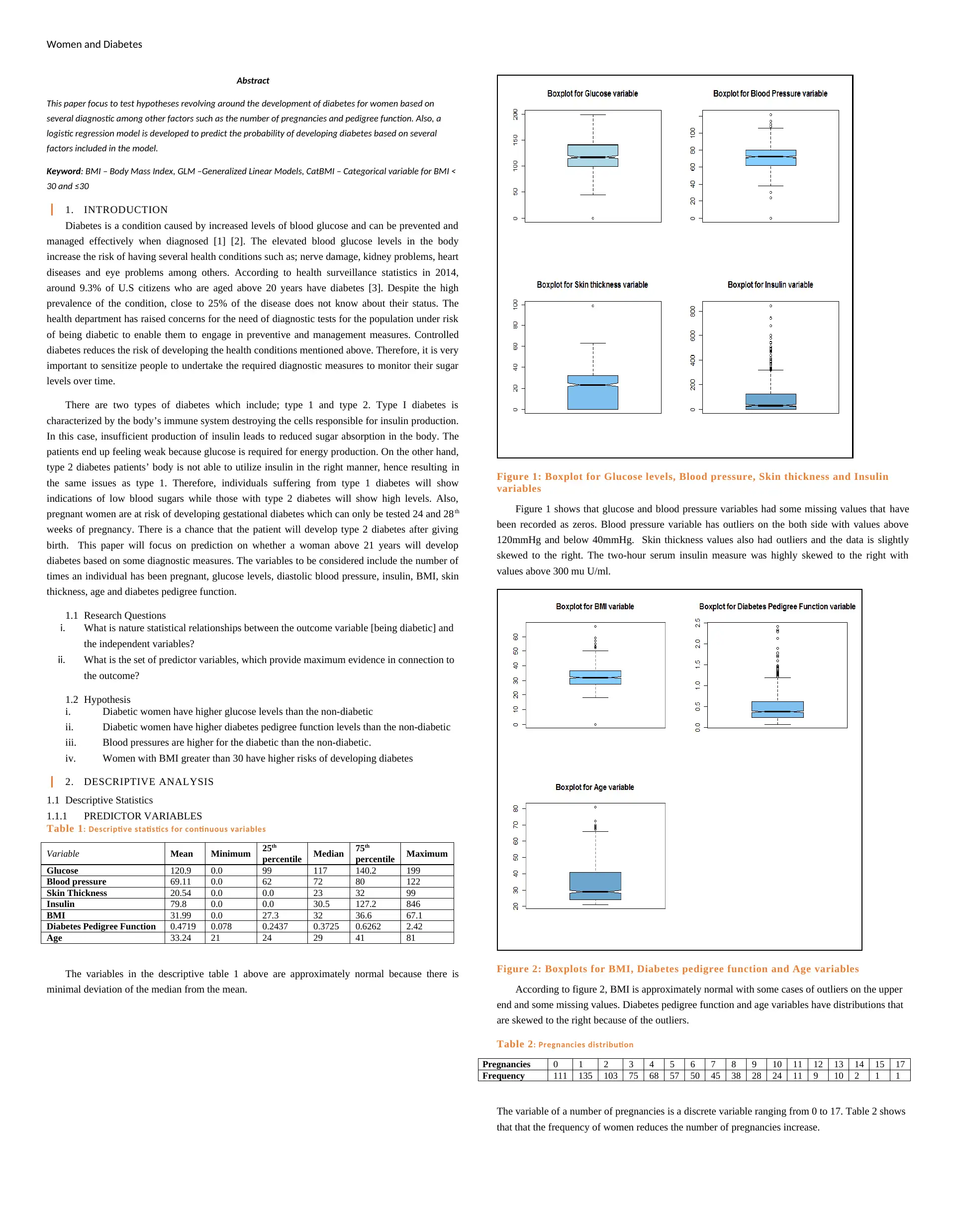
Table 1: Descriptive statistics for continuous variables
Variable Mean Minimum 25th
percentile Median 75th
percentile Maximum
Glucose 120.9 0.0 99 117 140.2 199
Blood pressure 69.11 0.0 62 72 80 122
Skin Thickness 20.54 0.0 0.0 23 32 99
Insulin 79.8 0.0 0.0 30.5 127.2 846
BMI 31.99 0.0 27.3 32 36.6 67.1
Diabetes Pedigree Function 0.4719 0.078 0.2437 0.3725 0.6262 2.42
Age 33.24 21 24 29 41 81
The variables in the descriptive table 1 above are approximately normal because there is
minimal deviation of the median from the mean.
Figure 1: Boxplot for Glucose levels, Blood pressure, Skin thickness and Insulin
variables
Figure 1 shows that glucose and blood pressure variables had some missing values that have
been recorded as zeros. Blood pressure variable has outliers on the both side with values above
120mmHg and below 40mmHg. Skin thickness values also had outliers and the data is slightly
skewed to the right. The two-hour serum insulin measure was highly skewed to the right with
values above 300 mu U/ml.
Figure 2: Boxplots for BMI, Diabetes pedigree function and Age variables
According to figure 2, BMI is approximately normal with some cases of outliers on the upper
end and some missing values. Diabetes pedigree function and age variables have distributions that
are skewed to the right because of the outliers.
Table 2: Pregnancies distribution
Pregnancies 0 1 2 3 4 5 6 7 8 9 10 11 12 13 14 15 17
Frequency 111 135 103 75 68 57 50 45 38 28 24 11 9 10 2 1 1
The variable of a number of pregnancies is a discrete variable ranging from 0 to 17. Table 2 shows
that that the frequency of women reduces the number of pregnancies increase.

Women and Diabetes
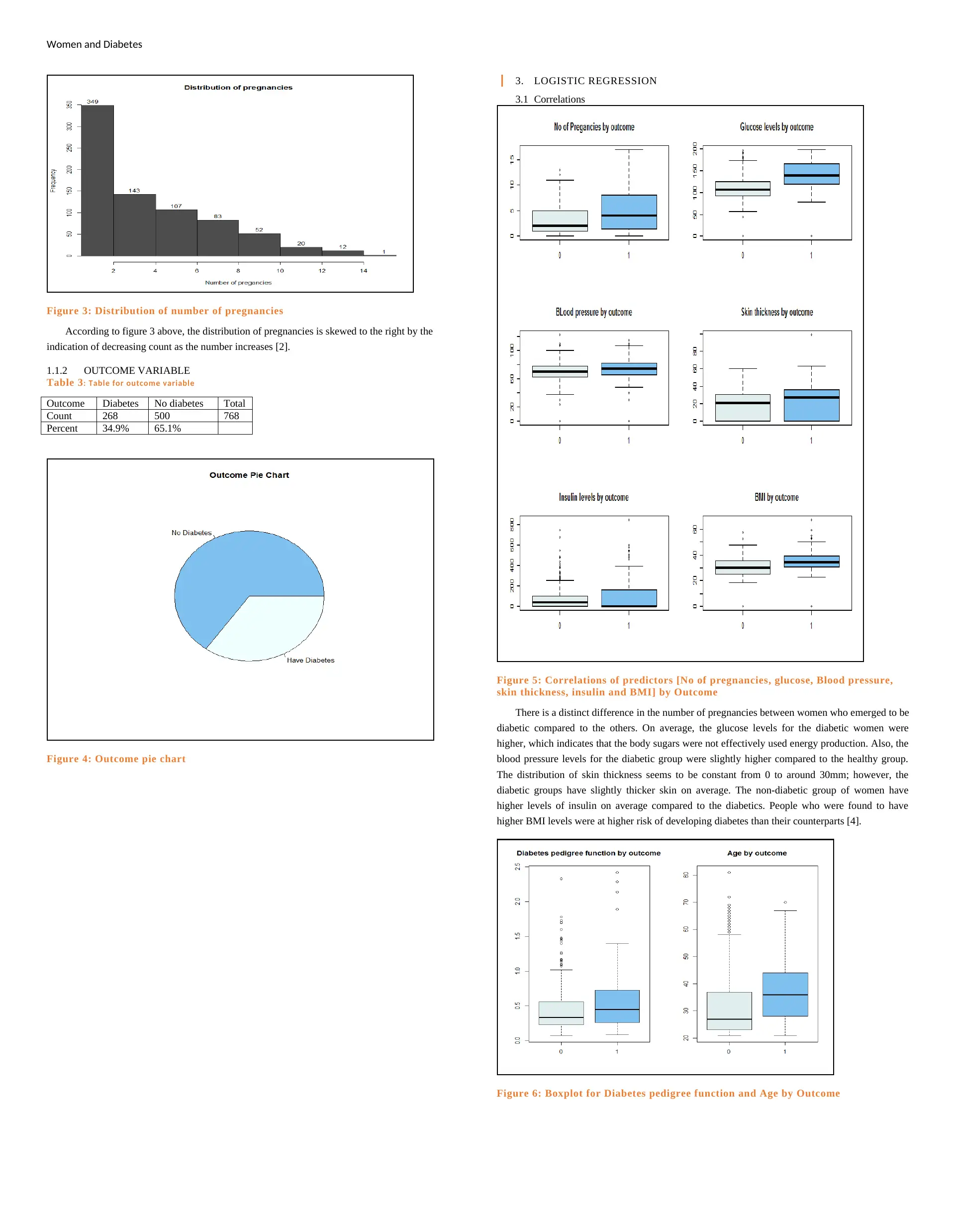
Figure 3: Distribution of number of pregnancies
According to figure 3 above, the distribution of pregnancies is skewed to the right by the
indication of decreasing count as the number increases [2].
1.1.2 OUTCOME VARIABLE
Table 3: Table for outcome variable
Outcome Diabetes No diabetes Total
Count 268 500 768
Percent 34.9% 65.1%
Figure 4: Outcome pie chart
3. LOGISTIC REGRESSION
3.1 Correlations
Figure 5: Correlations of predictors [No of pregnancies, glucose, Blood pressure,
skin thickness, insulin and BMI] by Outcome
There is a distinct difference in the number of pregnancies between women who emerged to be
diabetic compared to the others. On average, the glucose levels for the diabetic women were
higher, which indicates that the body sugars were not effectively used energy production. Also, the
blood pressure levels for the diabetic group were slightly higher compared to the healthy group.
The distribution of skin thickness seems to be constant from 0 to around 30mm; however, the
diabetic groups have slightly thicker skin on average. The non-diabetic group of women have
higher levels of insulin on average compared to the diabetics. People who were found to have
higher BMI levels were at higher risk of developing diabetes than their counterparts [4].
Figure 6: Boxplot for Diabetes pedigree function and Age by Outcome

Women and Diabetes
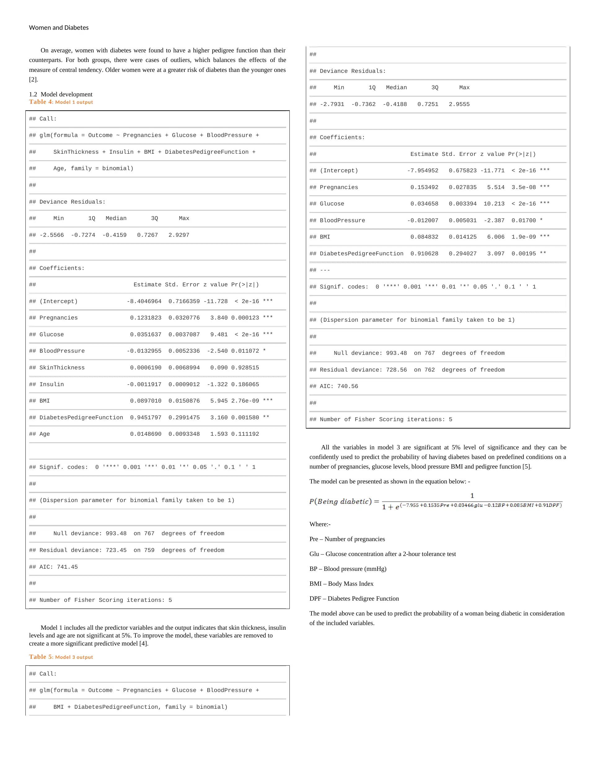
On average, women with diabetes were found to have a higher pedigree function than their
counterparts. For both groups, there were cases of outliers, which balances the effects of the
measure of central tendency. Older women were at a greater risk of diabetes than the younger ones
[2].
1.2 Model development
Table 4: Model 1 output
## Call:
## glm(formula = Outcome ~ Pregnancies + Glucose + BloodPressure +
## SkinThickness + Insulin + BMI + DiabetesPedigreeFunction +
## Age, family = binomial)
##
## Deviance Residuals:
## Min 1Q Median 3Q Max
## -2.5566 -0.7274 -0.4159 0.7267 2.9297
##
## Coefficients:
## Estimate Std. Error z value Pr(>|z|)
## (Intercept) -8.4046964 0.7166359 -11.728 < 2e-16 ***
## Pregnancies 0.1231823 0.0320776 3.840 0.000123 ***
## Glucose 0.0351637 0.0037087 9.481 < 2e-16 ***
## BloodPressure -0.0132955 0.0052336 -2.540 0.011072 *
## SkinThickness 0.0006190 0.0068994 0.090 0.928515
## Insulin -0.0011917 0.0009012 -1.322 0.186065
## BMI 0.0897010 0.0150876 5.945 2.76e-09 ***
## DiabetesPedigreeFunction 0.9451797 0.2991475 3.160 0.001580 **
## Age 0.0148690 0.0093348 1.593 0.111192
## Signif. codes: 0 '***' 0.001 '**' 0.01 '*' 0.05 '.' 0.1 ' ' 1
##
## (Dispersion parameter for binomial family taken to be 1)
##
## Null deviance: 993.48 on 767 degrees of freedom
## Residual deviance: 723.45 on 759 degrees of freedom
## AIC: 741.45
##
## Number of Fisher Scoring iterations: 5
Model 1 includes all the predictor variables and the output indicates that skin thickness, insulin
levels and age are not significant at 5%. To improve the model, these variables are removed to
create a more significant predictive model [4].
Table 5: Model 3 output
## Call:
## glm(formula = Outcome ~ Pregnancies + Glucose + BloodPressure +
## BMI + DiabetesPedigreeFunction, family = binomial)
##
## Deviance Residuals:
## Min 1Q Median 3Q Max
## -2.7931 -0.7362 -0.4188 0.7251 2.9555
##
## Coefficients:
## Estimate Std. Error z value Pr(>|z|)
## (Intercept) -7.954952 0.675823 -11.771 < 2e-16 ***
## Pregnancies 0.153492 0.027835 5.514 3.5e-08 ***
## Glucose 0.034658 0.003394 10.213 < 2e-16 ***
## BloodPressure -0.012007 0.005031 -2.387 0.01700 *
## BMI 0.084832 0.014125 6.006 1.9e-09 ***
## DiabetesPedigreeFunction 0.910628 0.294027 3.097 0.00195 **
## ---
## Signif. codes: 0 '***' 0.001 '**' 0.01 '*' 0.05 '.' 0.1 ' ' 1
##
## (Dispersion parameter for binomial family taken to be 1)
##
## Null deviance: 993.48 on 767 degrees of freedom
## Residual deviance: 728.56 on 762 degrees of freedom
## AIC: 740.56
##
## Number of Fisher Scoring iterations: 5
All the variables in model 3 are significant at 5% level of significance and they can be
confidently used to predict the probability of having diabetes based on predefined conditions on a
number of pregnancies, glucose levels, blood pressure BMI and pedigree function [5].
The model can be presented as shown in the equation below: -
Where:-
Pre – Number of pregnancies
Glu – Glucose concentration after a 2-hour tolerance test
BP – Blood pressure (mmHg)
BMI – Body Mass Index
DPF – Diabetes Pedigree Function
The model above can be used to predict the probability of a woman being diabetic in consideration
of the included variables.

Women and Diabetes
4. HYPOTHESIS TESTING
4.1 Diabetic women have higher glucose levels than the non-diabetic
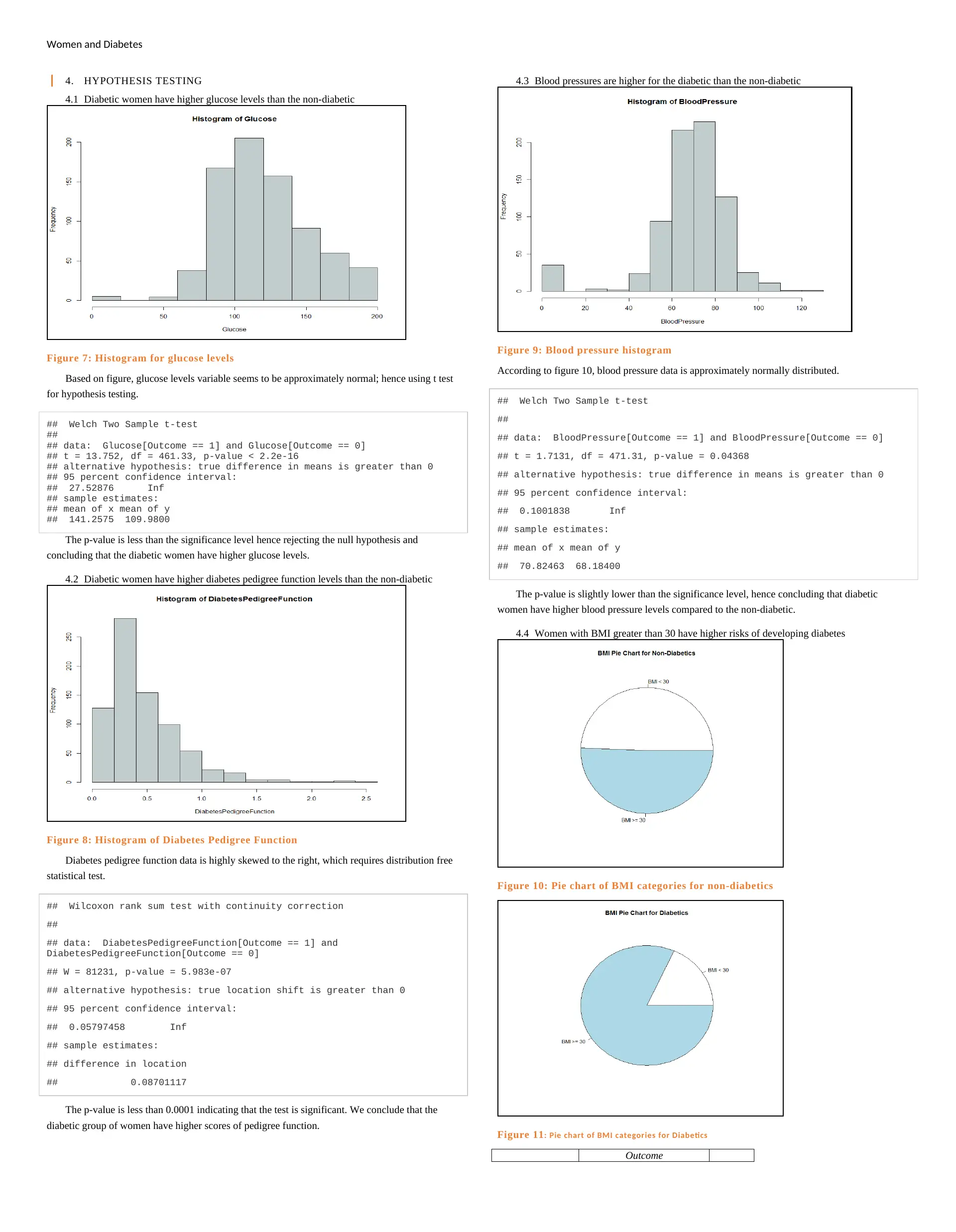
Figure 7: Histogram for glucose levels
Based on figure, glucose levels variable seems to be approximately normal; hence using t test
for hypothesis testing.
## Welch Two Sample t-test
##
## data: Glucose[Outcome == 1] and Glucose[Outcome == 0]
## t = 13.752, df = 461.33, p-value < 2.2e-16
## alternative hypothesis: true difference in means is greater than 0
## 95 percent confidence interval:
## 27.52876 Inf
## sample estimates:
## mean of x mean of y
## 141.2575 109.9800
The p-value is less than the significance level hence rejecting the null hypothesis and
concluding that the diabetic women have higher glucose levels.
4.2 Diabetic women have higher diabetes pedigree function levels than the non-diabetic
Figure 8: Histogram of Diabetes Pedigree Function
Diabetes pedigree function data is highly skewed to the right, which requires distribution free
statistical test.
## Wilcoxon rank sum test with continuity correction
##
## data: DiabetesPedigreeFunction[Outcome == 1] and
DiabetesPedigreeFunction[Outcome == 0]
## W = 81231, p-value = 5.983e-07
## alternative hypothesis: true location shift is greater than 0
## 95 percent confidence interval:
## 0.05797458 Inf
## sample estimates:
## difference in location
## 0.08701117
The p-value is less than 0.0001 indicating that the test is significant. We conclude that the
diabetic group of women have higher scores of pedigree function.
4.3 Blood pressures are higher for the diabetic than the non-diabetic
Figure 9: Blood pressure histogram
According to figure 10, blood pressure data is approximately normally distributed.
## Welch Two Sample t-test
##
## data: BloodPressure[Outcome == 1] and BloodPressure[Outcome == 0]
## t = 1.7131, df = 471.31, p-value = 0.04368
## alternative hypothesis: true difference in means is greater than 0
## 95 percent confidence interval:
## 0.1001838 Inf
## sample estimates:
## mean of x mean of y
## 70.82463 68.18400
The p-value is slightly lower than the significance level, hence concluding that diabetic
women have higher blood pressure levels compared to the non-diabetic.
4.4 Women with BMI greater than 30 have higher risks of developing diabetes
Figure 10: Pie chart of BMI categories for non-diabetics
Figure 11: Pie chart of BMI categories for Diabetics
Outcome

Women and Diabetes
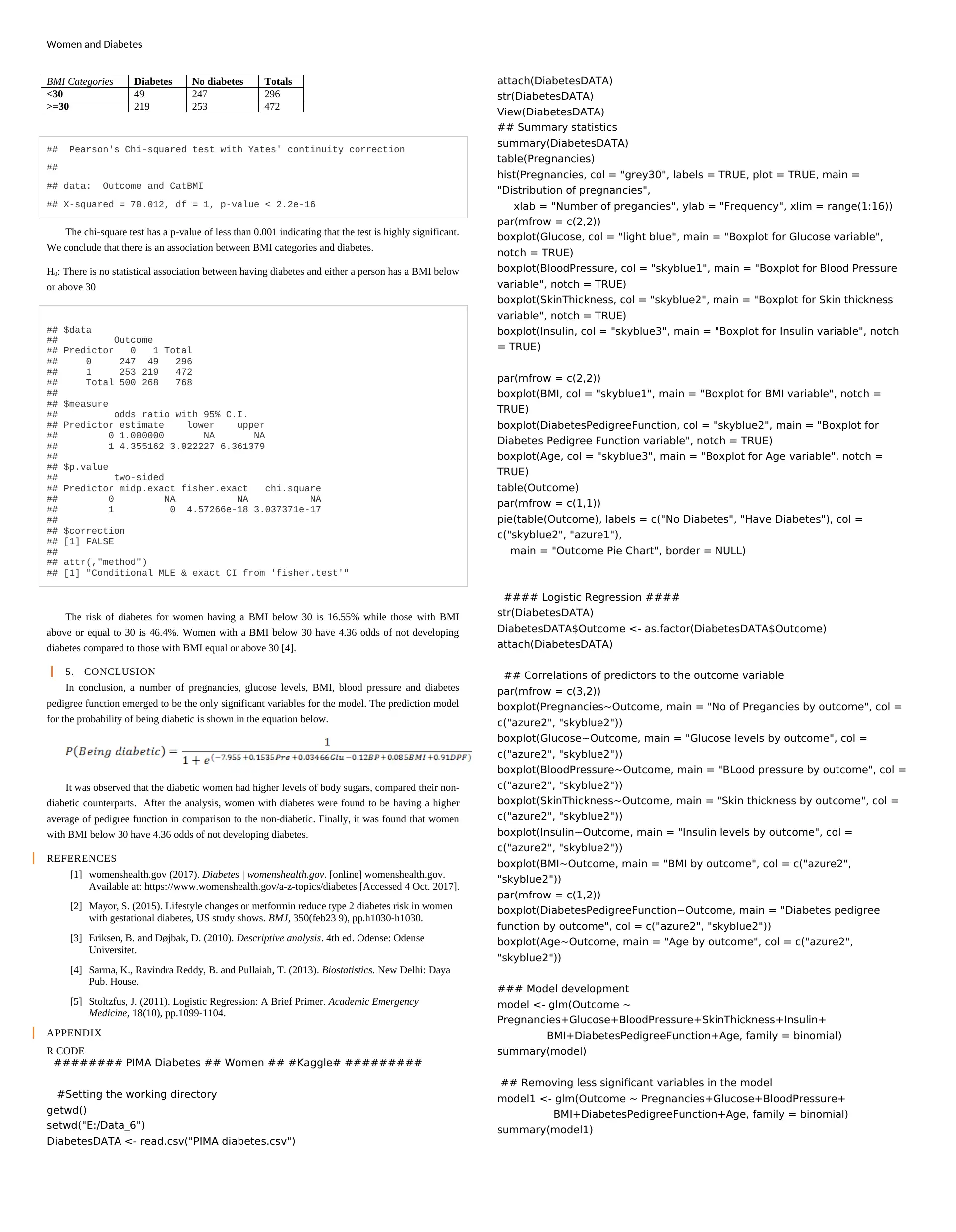
BMI Categories Diabetes No diabetes Totals
<30 49 247 296
>=30 219 253 472
## Pearson's Chi-squared test with Yates' continuity correction
##
## data: Outcome and CatBMI
## X-squared = 70.012, df = 1, p-value < 2.2e-16
The chi-square test has a p-value of less than 0.001 indicating that the test is highly significant.
We conclude that there is an association between BMI categories and diabetes.
H0: There is no statistical association between having diabetes and either a person has a BMI below
or above 30
## $data
## Outcome
## Predictor 0 1 Total
## 0 247 49 296
## 1 253 219 472
## Total 500 268 768
##
## $measure
## odds ratio with 95% C.I.
## Predictor estimate lower upper
## 0 1.000000 NA NA
## 1 4.355162 3.022227 6.361379
##
## $p.value
## two-sided
## Predictor midp.exact fisher.exact chi.square
## 0 NA NA NA
## 1 0 4.57266e-18 3.037371e-17
##
## $correction
## [1] FALSE
##
## attr(,"method")
## [1] "Conditional MLE & exact CI from 'fisher.test'"
The risk of diabetes for women having a BMI below 30 is 16.55% while those with BMI
above or equal to 30 is 46.4%. Women with a BMI below 30 have 4.36 odds of not developing
diabetes compared to those with BMI equal or above 30 [4].
5. CONCLUSION
In conclusion, a number of pregnancies, glucose levels, BMI, blood pressure and diabetes
pedigree function emerged to be the only significant variables for the model. The prediction model
for the probability of being diabetic is shown in the equation below.
It was observed that the diabetic women had higher levels of body sugars, compared their non-
diabetic counterparts. After the analysis, women with diabetes were found to be having a higher
average of pedigree function in comparison to the non-diabetic. Finally, it was found that women
with BMI below 30 have 4.36 odds of not developing diabetes.
REFERENCES
[1] womenshealth.gov (2017). Diabetes | womenshealth.gov. [online] womenshealth.gov.
Available at: https://www.womenshealth.gov/a-z-topics/diabetes [Accessed 4 Oct. 2017].
[2] Mayor, S. (2015). Lifestyle changes or metformin reduce type 2 diabetes risk in women
with gestational diabetes, US study shows. BMJ, 350(feb23 9), pp.h1030-h1030.
[3] Eriksen, B. and Døjbak, D. (2010). Descriptive analysis. 4th ed. Odense: Odense
Universitet.
[4] Sarma, K., Ravindra Reddy, B. and Pullaiah, T. (2013). Biostatistics. New Delhi: Daya
Pub. House.
[5] Stoltzfus, J. (2011). Logistic Regression: A Brief Primer. Academic Emergency
Medicine, 18(10), pp.1099-1104.
APPENDIX
R CODE
######## PIMA Diabetes ## Women ## #Kaggle# #########
#Setting the working directory
getwd()
setwd("E:/Data_6")
DiabetesDATA <- read.csv("PIMA diabetes.csv")
attach(DiabetesDATA)
str(DiabetesDATA)
View(DiabetesDATA)
## Summary statistics
summary(DiabetesDATA)
table(Pregnancies)
hist(Pregnancies, col = "grey30", labels = TRUE, plot = TRUE, main =
"Distribution of pregnancies",
xlab = "Number of pregancies", ylab = "Frequency", xlim = range(1:16))
par(mfrow = c(2,2))
boxplot(Glucose, col = "light blue", main = "Boxplot for Glucose variable",
notch = TRUE)
boxplot(BloodPressure, col = "skyblue1", main = "Boxplot for Blood Pressure
variable", notch = TRUE)
boxplot(SkinThickness, col = "skyblue2", main = "Boxplot for Skin thickness
variable", notch = TRUE)
boxplot(Insulin, col = "skyblue3", main = "Boxplot for Insulin variable", notch
= TRUE)
par(mfrow = c(2,2))
boxplot(BMI, col = "skyblue1", main = "Boxplot for BMI variable", notch =
TRUE)
boxplot(DiabetesPedigreeFunction, col = "skyblue2", main = "Boxplot for
Diabetes Pedigree Function variable", notch = TRUE)
boxplot(Age, col = "skyblue3", main = "Boxplot for Age variable", notch =
TRUE)
table(Outcome)
par(mfrow = c(1,1))
pie(table(Outcome), labels = c("No Diabetes", "Have Diabetes"), col =
c("skyblue2", "azure1"),
main = "Outcome Pie Chart", border = NULL)
#### Logistic Regression ####
str(DiabetesDATA)
DiabetesDATA$Outcome <- as.factor(DiabetesDATA$Outcome)
attach(DiabetesDATA)
## Correlations of predictors to the outcome variable
par(mfrow = c(3,2))
boxplot(Pregnancies~Outcome, main = "No of Pregancies by outcome", col =
c("azure2", "skyblue2"))
boxplot(Glucose~Outcome, main = "Glucose levels by outcome", col =
c("azure2", "skyblue2"))
boxplot(BloodPressure~Outcome, main = "BLood pressure by outcome", col =
c("azure2", "skyblue2"))
boxplot(SkinThickness~Outcome, main = "Skin thickness by outcome", col =
c("azure2", "skyblue2"))
boxplot(Insulin~Outcome, main = "Insulin levels by outcome", col =
c("azure2", "skyblue2"))
boxplot(BMI~Outcome, main = "BMI by outcome", col = c("azure2",
"skyblue2"))
par(mfrow = c(1,2))
boxplot(DiabetesPedigreeFunction~Outcome, main = "Diabetes pedigree
function by outcome", col = c("azure2", "skyblue2"))
boxplot(Age~Outcome, main = "Age by outcome", col = c("azure2",
"skyblue2"))
### Model development
model <- glm(Outcome ~
Pregnancies+Glucose+BloodPressure+SkinThickness+Insulin+
BMI+DiabetesPedigreeFunction+Age, family = binomial)
summary(model)
## Removing less significant variables in the model
model1 <- glm(Outcome ~ Pregnancies+Glucose+BloodPressure+
BMI+DiabetesPedigreeFunction+Age, family = binomial)
summary(model1)

Women and Diabetes
model3 <- glm(Outcome ~ Pregnancies+Glucose+BloodPressure+
BMI+DiabetesPedigreeFunction, family = binomial)
summary(model3)
par(mfrow = c(2,2))
plot(model3)
## Hypothesis testing
#Diabetic women have higher glucose levels than the non-diabetic
par(mfrow= c(1,1))
hist(Glucose, col = "azure3")
t.test(Glucose[Outcome == 1], Glucose[Outcome == 0], paired = FALSE,
alternative = "greater")
#Diabetic women have higher diabetes pedigree function levels than the non-
diabetic
hist(DiabetesPedigreeFunction, col = "azure3")
wilcox.test(DiabetesPedigreeFunction[Outcome == 1],
DiabetesPedigreeFunction[Outcome == 0],
paired = FALSE, mu=0, conf.int = TRUE, alternative = "greater")
#Blood pressures are higher for the diabetic than the non-diabetic
hist(BloodPressure, col = "azure3", probability = TRUE)
t.test(BloodPressure[Outcome == 1], BloodPressure[Outcome == 0], paired =
FALSE, alternative = "greater")
#Women with BMI greater than 30 have higher risks of developing diabetes
#creating a dummy variable for BMI < 30 = 0 and 1 otherwise
DiabetesDATA$CatBMI <- as.factor(ifelse(BMI<30, 0, 1))
attach(DiabetesDATA)
table(CatBMI)
par(mfrow = c(1,1))
pie(table(CatBMI[Outcome == 0]), labels = c("BMI < 30", "BMI >= 30"), main
= "BMI Pie Chart for Non-Diabetics")
pie(table(CatBMI[Outcome == 1]), labels = c("BMI < 30", "BMI >= 30"), main
= "BMI Pie Chart for Diabetics")
library(epitools)
tab <- table(CatBMI, Outcome)
epitab(CatBMI, Outcome)
chisq.test(Outcome, CatBMI, correct = TRUE)
oddsratio.fisher(CatBMI, Outcome)