ME108, Semester 1, 2019/2020: Piping Network Analysis using MATLAB
VerifiedAdded on 2022/08/26
|8
|1399
|14
Practical Assignment
AI Summary
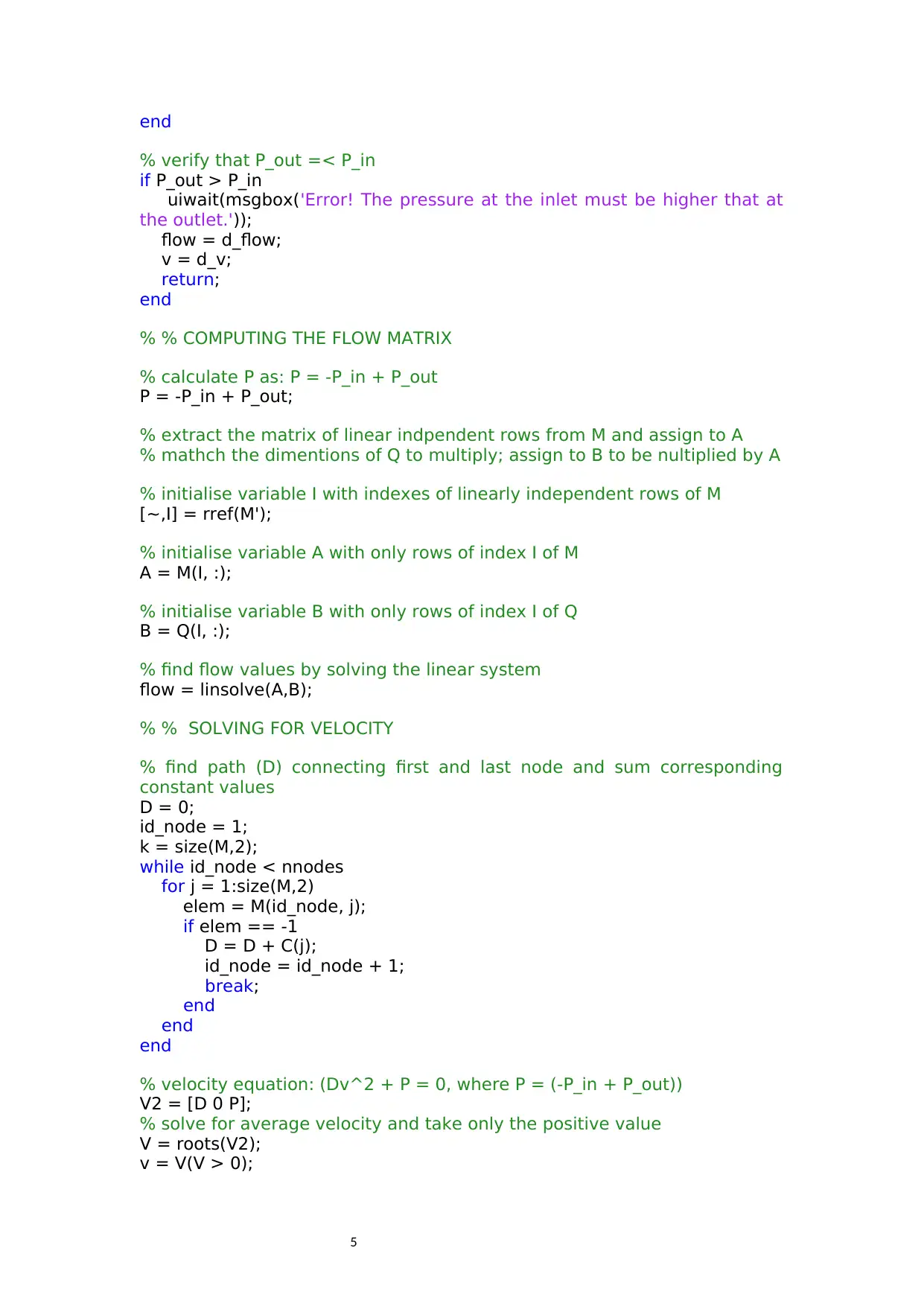
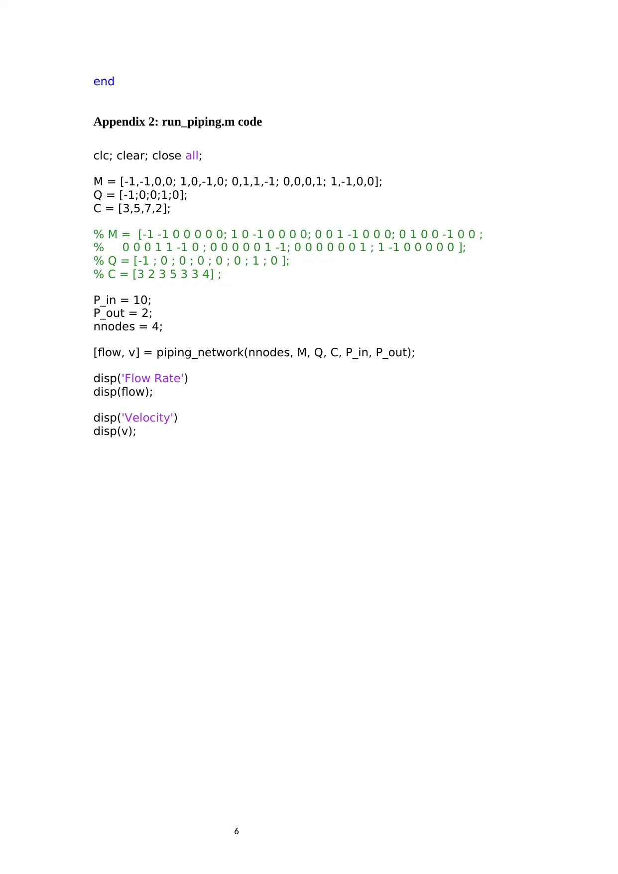
This assignment presents a MATLAB-based solution for analyzing a piping network system. The objective is to determine flow rates at various nodes and the average flow velocity, governed by a set of equations and constraints represented in matrix and vector forms. The solution utilizes MATLAB, employing a function within a .m file to ensure reusability and facilitate validation against provided data. The document includes the MATLAB code (piping_network.m and run_piping.m), along with validation results and test results using actual data. The code is well-commented for readability. The solution addresses the given parameters: flow rate matrix (N), vector (C), matrix (Q), and pressure values, demonstrating the application of linear algebra principles. The appendices contain the complete MATLAB code, and figures illustrate the validation and test results, offering a comprehensive overview of the implemented solution for mechanical engineering students.


1 out of 8

Your All-in-One AI-Powered Toolkit for Academic Success.
+13062052269
info@desklib.com
Available 24*7 on WhatsApp / Email
![[object Object]](/_next/static/media/star-bottom.7253800d.svg)
Copyright © 2020–2026 A2Z Services. All Rights Reserved. Developed and managed by ZUCOL.