Power System Frequency Control using Simplified Models Analysis

This assignment delves into the intricacies of power system frequency control, examining how different generation source mixes affect performance. The analysis encompasses synchronous and asynchronous generation, exploring the impact of governor droop and inertia constants. The student utilized MATLAB Simulink to simulate system responses, derive equations of motion, and compare simulated results with mathematical derivations. The assignment investigates the effects of adding governors to synchronous generators and the resulting system-frequency response with primary frequency control. Furthermore, the study explores factors influencing system frequency response, such as inertia constant and governor droop, and evaluates the effects of reducing the proportion of online synchronous generation capacity. The conclusion summarizes the key findings and highlights the influence of various parameters on system frequency stability and control.

POWER SYSTEM FREQUENCY CONTROL USING SIMPLIFIED MODELS.
BY (STUDENT NAME)
CLASS (COURSE) NAME:
TUTOR (PROFESSOR):
SCHOOL NAME:
THE CITY/STATE:
DATE:

Table of Contents
Introduction...................................................................................................................... 3
Answers to given questions............................................................................................. 4
Part a) Equation of motion............................................................................................4
Part b) System-frequency response without frequency-control....................................6
Part c) Compare the simulated response with mathematically derived response.........7
Part d) Addition of governors to synchronous generators.............................................8
Part e): System-frequency response with primary frequency control..........................11
Part f) factors influencing system frequency response...............................................13
Conclusion..................................................................................................................... 14

Introduction.
The aim of this assignment is to investigate how a system frequency control system
performs as the mix of generation sources are varied. The performance for different proportions
of synchronous and asynchronous generation is performed, to how the frequency control
systems performs for different proportions of generation with frequency control using total online
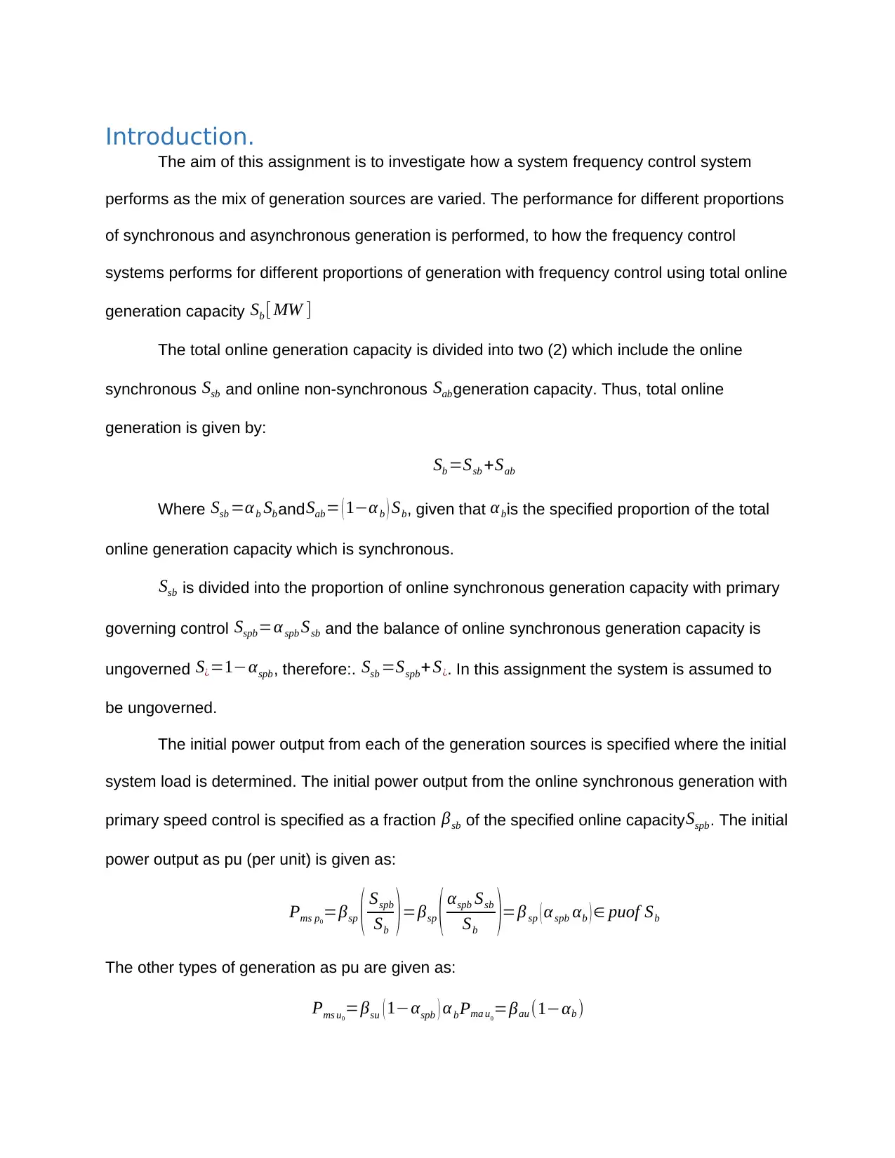
generation capacity Sb [ MW ]
The total online generation capacity is divided into two (2) which include the online
synchronous Ssb and online non-synchronous Sabgeneration capacity. Thus, total online
generation is given by:
Sb =Ssb +Sab
Where Ssb =αb SbandSab= ( 1−αb ) Sb, given that α bis the specified proportion of the total
online generation capacity which is synchronous.
Ssb is divided into the proportion of online synchronous generation capacity with primary
governing control Sspb=α spb Ssb and the balance of online synchronous generation capacity is
ungoverned S¿=1−αspb, therefore:. Ssb =Sspb+ S¿. In this assignment the system is assumed to
be ungoverned.
The initial power output from each of the generation sources is specified where the initial
system load is determined. The initial power output from the online synchronous generation with
primary speed control is specified as a fraction βsb of the specified online capacity Sspb. The initial
power output as pu (per unit) is given as:
Pms p0
=βsp ( Sspb
Sb )=βsp ( αspb Ssb
Sb )=β sp ( α spb αb ) ∈ puof Sb
The other types of generation as pu are given as:
Pms u0
=βsu ( 1−αspb ) αbPma u0
=βau (1−αb )

Where the initial power output from the synchronous generation sources is Pm s0
=Pms u0
+ Pmau0
and from the asynchronous generation sources isPm a0
=Pmau0 , thus, the total output generation
sources are Pm0
=Pm s0
+ Pm a0. Therefore, to define the initial steady-state operating point of the
system it is required to specify βsp , βau∧β su
The inertia constant of online synchronous generation limits the rate of change of
frequency, and it is converted to pu as: H=H s ( Ssb
Sb )=αb Hs
The system load is linearly dependent on the system-frequency perturbation as:
Pl ( f ) =Pl0
( 1+D ∆ f )
Where Pl0the initial steady-state value of the load f =f 0 ( 1+∆ f ) is the system frequency, ∆ f is
per-unit system-frequency perturbation and f 0=50 Hzis the nominal frequency of the system
Answers to given questions
Part a) Equation of motion
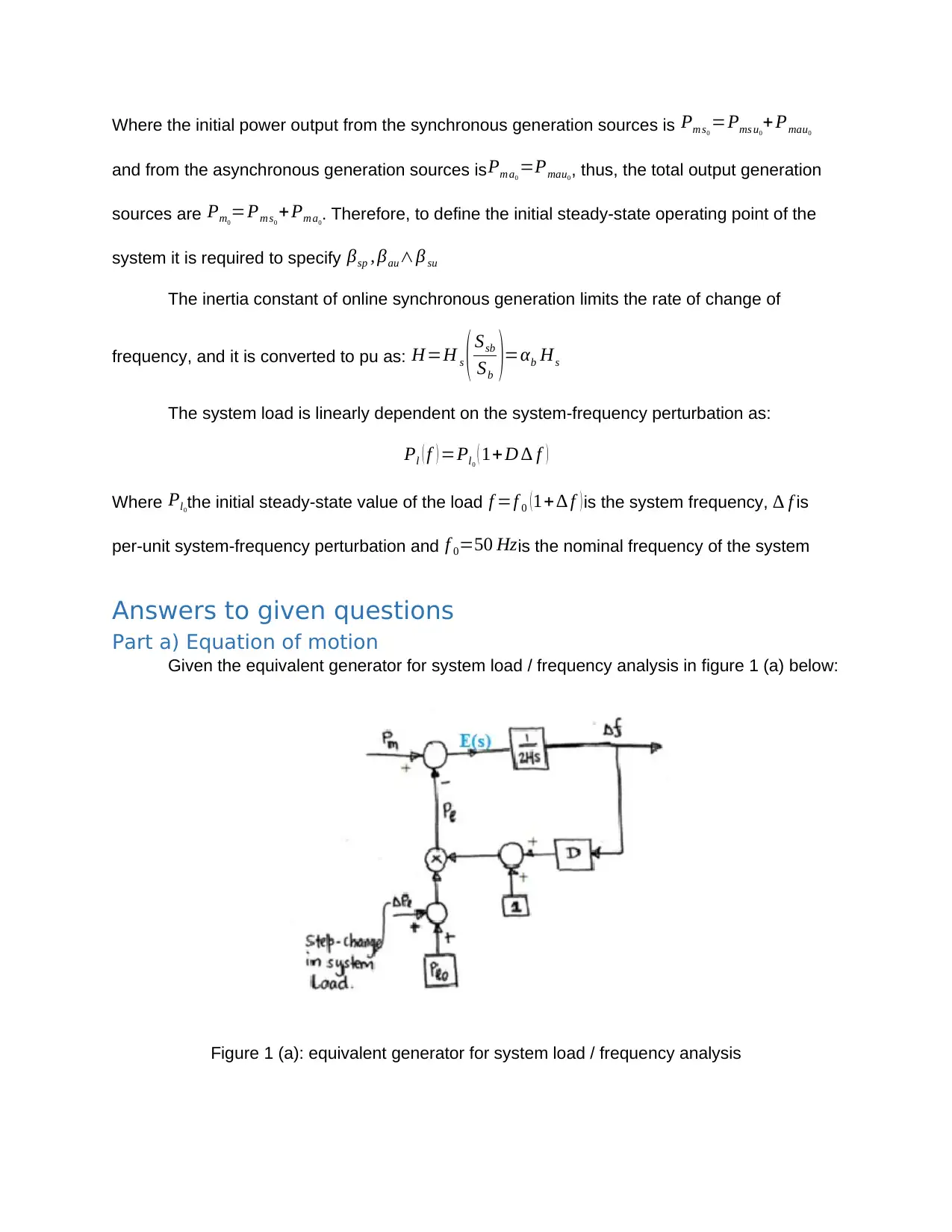
Given the equivalent generator for system load / frequency analysis in figure 1 (a) below:
Figure 1 (a): equivalent generator for system load / frequency analysis

The derivation of general equations for the initial-values of the outputs on the integrator(s) in the
system in figure 1. From the figure we can deduct the following equations
∆ f = E ( s )
2 Hs (i)E ( s )=Pm−Pl (ii) Pe=( ( Plo+ ∆ Pl ) + ( D+1 ) )∆ f (iii)
Combining equation (ii) and (ii):
E ( s )=Pm−( ( Plo+ ∆ Pl ) + ( D+1 )) ∆ f (iv )
Eliminating E(s) from equation (i) using equation (iv) gives
∆ f =Pm−¿ ¿
Making ∆ f the subject of the formula:
∆ f = 1
2 Hs ( pm− ( Plo+ ∆ Pl )
D+1 ) ( vi )
Let Plo+∆ Pl
D+ 1 = pl
∆ f = 1
2 Hs ( pm− pl )(vii)
The mathematical modelling block diagram of load can be represented as in figure 1 (b) below
Figure 1 (b): The mathematical modelling block diagram
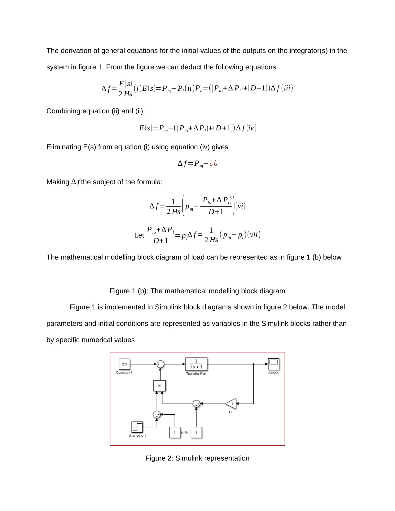
Figure 1 is implemented in Simulink block diagrams shown in figure 2 below. The model
parameters and initial conditions are represented as variables in the Simulink blocks rather than
by specific numerical values
Figure 2: Simulink representation

Part b) System-frequency response without frequency-control.
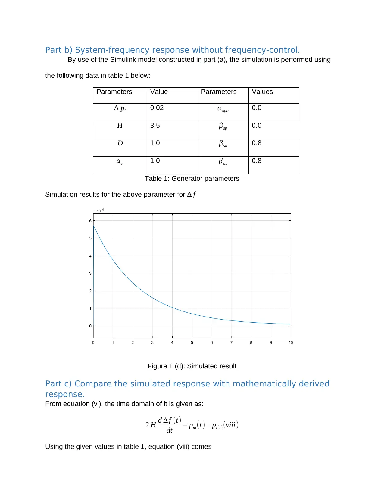
By use of the Simulink model constructed in part (a), the simulation is performed using
the following data in table 1 below:
Parameters Value Parameters Values
∆ pl 0.02 α spb 0.0
H 3.5 βsp 0.0
D 1.0 βsu 0.8
α b 1.0 βau 0.8
Table 1: Generator parameters
Simulation results for the above parameter for ∆ f
Figure 1 (d): Simulated result
Part c) Compare the simulated response with mathematically derived
response.
From equation (vi), the time domain of it is given as:
2 H d ∆ f (t)
dt = pm (t )− pl(t )(viii )
Using the given values in table 1, equation (viii) comes

7 d ∆ f
dt =2 pm ( t ) −pl ( t ) (ix)
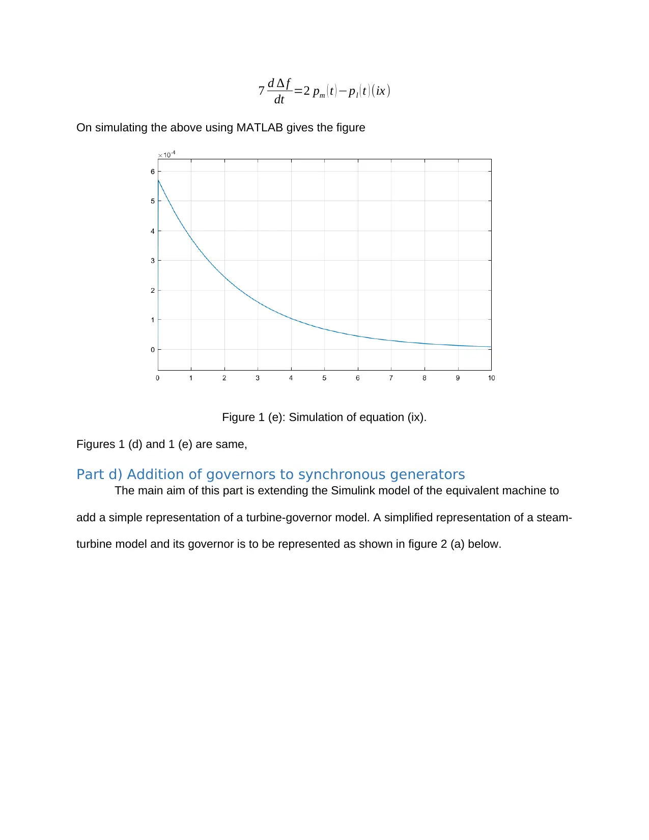
On simulating the above using MATLAB gives the figure
Figure 1 (e): Simulation of equation (ix).
Figures 1 (d) and 1 (e) are same,
Part d) Addition of governors to synchronous generators
The main aim of this part is extending the Simulink model of the equivalent machine to
add a simple representation of a turbine-governor model. A simplified representation of a steam-
turbine model and its governor is to be represented as shown in figure 2 (a) below.

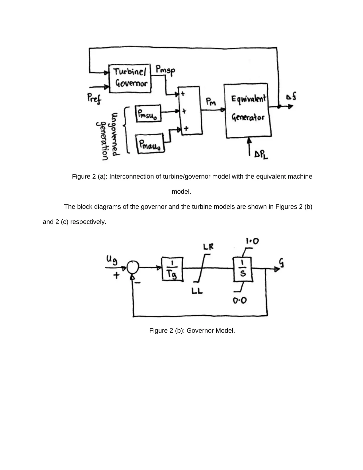
Figure 2 (a): Interconnection of turbine/governor model with the equivalent machine
model.
The block diagrams of the governor and the turbine models are shown in Figures 2 (b)
and 2 (c) respectively.
Figure 2 (b): Governor Model.

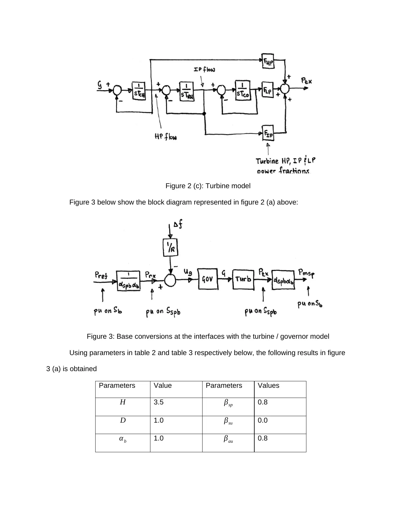
Figure 2 (c): Turbine model
Figure 3 below show the block diagram represented in figure 2 (a) above:
Figure 3: Base conversions at the interfaces with the turbine / governor model
Using parameters in table 2 and table 3 respectively below, the following results in figure
3 (a) is obtained
Parameters Value Parameters Values
H 3.5 βsp 0.8
D 1.0 βsu 0.0
α b 1.0 βau 0.8

α spb 1.0
Table 2: Base case turbine-governor study – equivalent generator parameters.
Parameters Value Parameters Values
R 0.05 T RH ( s) 7.0
T g ( s) 0.3 T CO( s) 0.5
LR ( pu
s ) 0.1 FHP (s) 0.3
¿ ( pu
s ) -1.0 FIP( s) 0.3
T CH (s) 0.3 FLP (s) 0.4
Table 3: Base case turbine-governor study –equivalent turbine-governor model
From the parameters above:
Pms u0
=βsu ( 1−αspb ) α b=0.0 ( 1−1 ) ×1=0Pma u0
=βau ( 1−ab )=0.8 ( 1−1 )=0 Pm 0=0
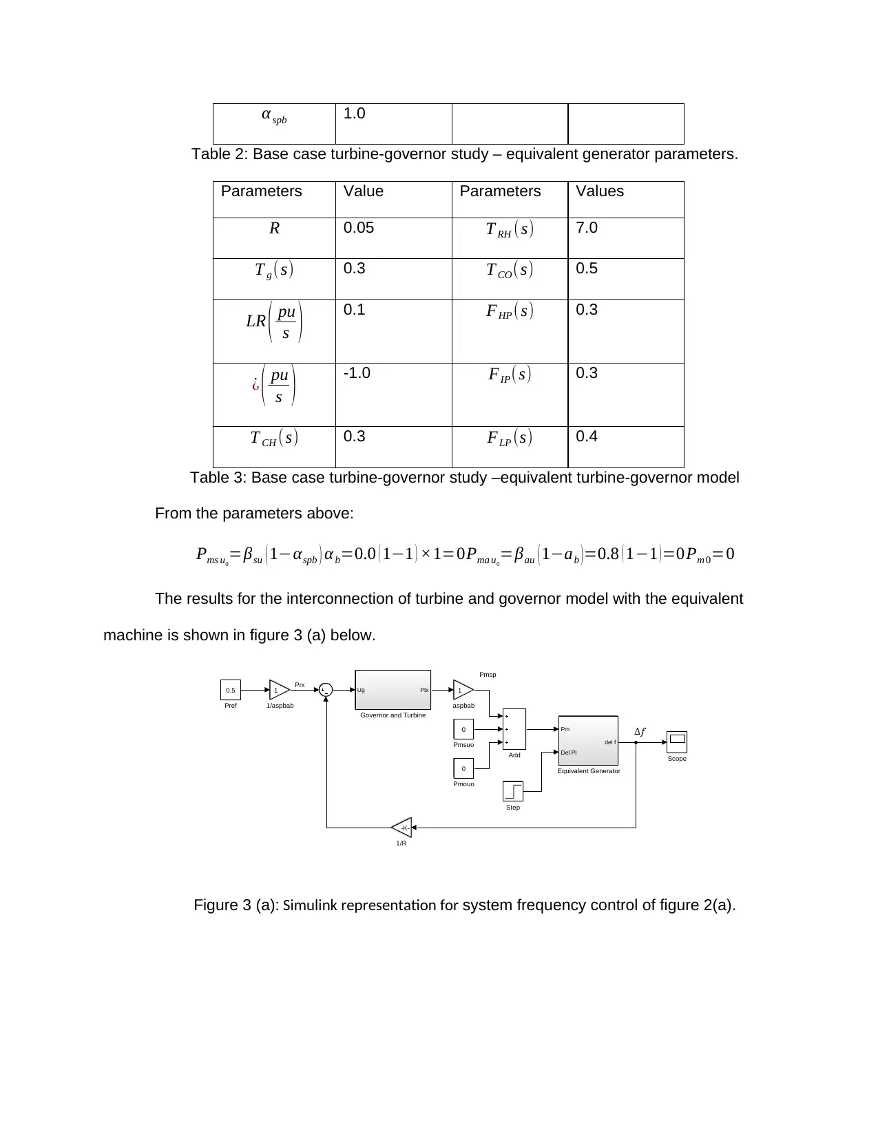
The results for the interconnection of turbine and governor model with the equivalent
machine is shown in figure 3 (a) below.
Prx
Pmsp
Pm
Del Pl
del f
Equivalent Generator
Ug Ptx
Governor and Turbine
1
1/aspbab
1
aspbab
0.5
Pref
Add
0
Pmouo
0
Pmsuo
Step
-K-
1/R
Scope
Figure 3 (a): Simulink representation for system frequency control of figure 2(a).

Part e): System-frequency response with primary frequency control.
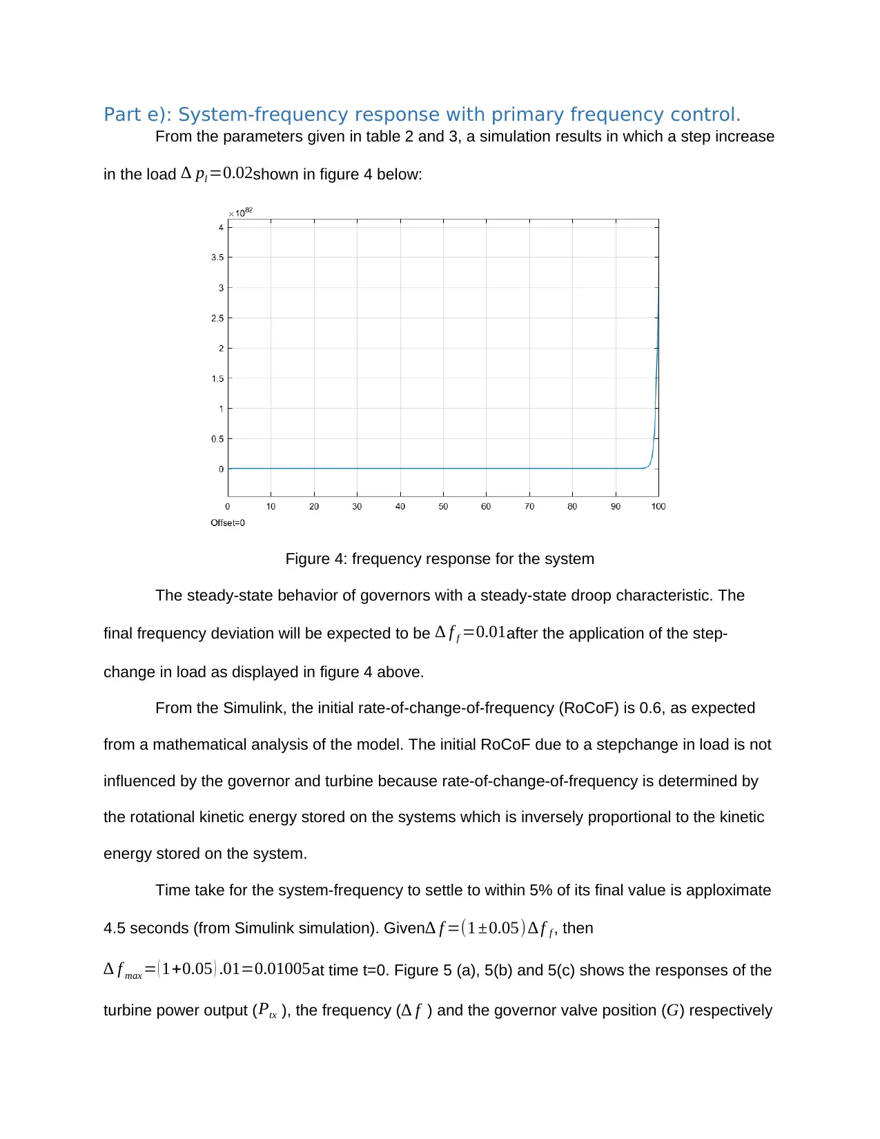
From the parameters given in table 2 and 3, a simulation results in which a step increase
in the load ∆ pl =0.02shown in figure 4 below:
Figure 4: frequency response for the system
The steady-state behavior of governors with a steady-state droop characteristic. The
final frequency deviation will be expected to be ∆ f f =0.01after the application of the step-
change in load as displayed in figure 4 above.
From the Simulink, the initial rate-of-change-of-frequency (RoCoF) is 0.6, as expected
from a mathematical analysis of the model. The initial RoCoF due to a stepchange in load is not
influenced by the governor and turbine because rate-of-change-of-frequency is determined by
the rotational kinetic energy stored on the systems which is inversely proportional to the kinetic
energy stored on the system.
Time take for the system-frequency to settle to within 5% of its final value is apploximate
4.5 seconds (from Simulink simulation). Given∆ f =(1 ±0.05)∆ f f , then
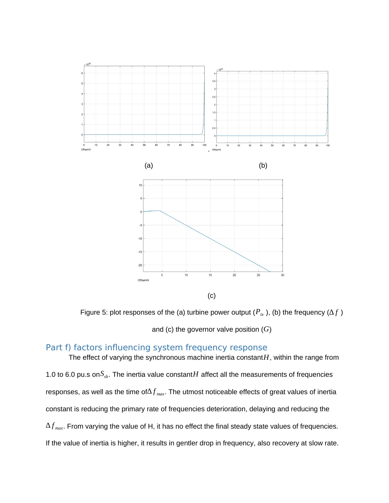
∆ f max = ( 1+0.05 ) .01=0.01005at time t=0. Figure 5 (a), 5(b) and 5(c) shows the responses of the
turbine power output ( Ptx ), the frequency ( ∆ f ) and the governor valve position (G) respectively

.
(a) (b)
(c)
Figure 5: plot responses of the (a) turbine power output (Ptx ), (b) the frequency (∆ f )
and (c) the governor valve position (G)
Part f) factors influencing system frequency response
The effect of varying the synchronous machine inertia constant H , within the range from
1.0 to 6.0 pu.s on Ssb. The inertia value constant H affect all the measurements of frequencies
responses, as well as the time of∆ f max. The utmost noticeable effects of great values of inertia
constant is reducing the primary rate of frequencies deterioration, delaying and reducing the
∆ f max. From varying the value of H, it has no effect the final steady state values of frequencies.
If the value of inertia is higher, it results in gentler drop in frequency, also recovery at slow rate.