Predicting Flank Wear of Cemented Carbide ISO P10
VerifiedAdded on 2022/12/27
|17
|4290
|1
AI Summary
This study focuses on predicting the flank wear of cemented carbide ISO P10 in turning of AISI 1045 steel. The analysis explores the relationship between tool wear and cutting parameters, and discusses the economic consequences of tool replacement. The study provides insights for optimizing the turning process to achieve desired product quality and reduce production costs.
Contribute Materials
Your contribution can guide someone’s learning journey. Share your
documents today.
Predicting Flank Wear of Cemented Carbide ISO P10
I. INTRODUCTION
Manufacturing companies similar to any other business aim at reducing the cost of
production in order to expand the profit margin in the current competitive business world.
The companies purchase machines which make it possible to produce finished products. For
example, an iron rod manufacturing company must purchase a cutting tool which they expect
to use for some time before replacing the components. In this sense, tool wear results in
replacement meaning making new orders and thus spending more. In this paper, a case of a
company dealing in turning of AISI 1045 using ISO P10 tool is considered for the analysis.
Tool wear calls for a replacement since degraded tools require more energy to operate and
might result in increased energy consumption. Thus, the economic consequence of replacing
a cutting tool comes with economic decision-making aspects [11].
According to Lopes [7], wear is undesirable deterioration of an element through the
removal of particles from a workpiece. Tool deformation is a tribological phenomenon
common with frequent machining resulting from increasing in surface irregularity [7]. The
parameters which affect the product quality and production cost include feed rate, cutting
speed and depth of cut. The major reason for optimizing turning process is to minimize
vibrations thus energy generated which cause increased tool wear [8]. Therefore, it is of
importance for the turning technique to attain optimal levels of the three parameters (cutting
speed, cutting depth and feed rate) in order to simultaneously achieve desired product quality,
reduced idle time and reduced cost of production [10]. According to [14], [12] and [4], the
cost of machining has a strong positive relationship with tool wear specifically in HSS cutting
tool.
Secure Best Marks with AI Grader
Need help grading? Try our AI Grader for instant feedback on your assignments.
II. METHOD AND DATA
AISI 1045 is medium tensile steel supplied in normalized condition or the black hot
rolled condition with has a tensile strength of between 570 - 700 MPa and Brinell hardness
ranging between 170 and 210 [1]. The approach used in the prediction of flank wear of AISI
1045 replicates the work done by Okokpujie et al. [16] titled “Experimental data-set for
prediction of tool wear during turning of Al-1061 alloy by high-speed steel cutting tools".
The data used for this project was obtained from the experimental data performed by Lopes
et al. [7]. The experiment collected data of end finishing end milling operations of AISI steel.
Therefore, instead of predicting Al-1061 tool wear the data on AISI 1045 is used to predict
flank wear of HSS used in the end finishing of AISI 1045.
The milling experiments were performed in a FADAL vertical machining center,
model VMC 15, with a maximum spindle rotation of 7500 RPM. The main motor of the
machine is the rate at 15 kW of power [7]. The cutting fluid used was synthetic oil Quimatic
MEII, and the tool overhang was 60 mm. A positive end mill tool, code R390-025A25-11M
with an entering angle of 90% and 25mm diameter. The tool had a medium step with three
inserts. In the experiment, three rectangular inserts with an edge length of 11 cm each were
used (Selvaraj & Chandramohan, 2010). The material of the tool used was cemented carbide
ISO P10 coated with TiN and TiCN through the PVD process with coating hardness of
approximately 3000 HV3 [7]. The tool's substrate hardness was estimated at 1650HV3 with
grain size less than 1μm. The work material used for the experiment was a rectangular block
with square cross-section 100mm and length of 300mm AISI 1045 medium tensile steel with
an estimated hardness of 180 HB [7].
The experiment was performed at the Federal University at Itajubá, Laboratory of
Mechanics. Measurements of the tool flank wear (VBmax) (fw) were captured with an optical
microscope (magnification 45X) with images acquired by a coupled digital camera. The
criteria adopted as the end of tool life was flank wear of approximately VBmax = 0.30 mm
[7]. The entire data set for 82 experiments was used to develop the prediction model. The
machining parameters such as feed rate of 0.01, 0.10, 0.15, 0.20 and 0.29 mm/tooth, and
radial depth of cut of 12.26, 15, 16.50, 18.00, and 20.74 mm and cutting speed of 254,300,
325, 350, and 396 m/min, was used as control factors during the finishing end milling
operation of AISI 1045 steel in order to predict flank wear, and to determine the effects of the
cutting parameters on the tool wear.
In this paper, the results were used to develop a model for the prediction of the tool
flank wear. Similar to Okokpujie et al. [16] data brief, least squares were used to estimate the
mathematical model presented in equation (1).

III. MATHEMATICAL MODEL AND COMPOSITION OF THE MATERIALS
According to Ramesh, Karunamoorthy & Palanikumar [13], the relationship between
tool wear and cutting parameters takes the form shown in equation (1).
TW max =K . V x . F y . Rz (1)
Where:
K is a constant
x, y, and z are the power equations
V is the cutting speed
F is the feed rate
R is the radial depth of cut.
Equation (1) is in the non-liner form thus least squares method would not be possible
therefore following the transformation procedure used by Okokpujie & Okonkwo [9]
equation is transformed using base 10 logarithm to equation (2).
log T W max=log K + x . log V + y . log F+ z . log R (2)
For simplification purposes, the equation is further transformed to
Y = β0 + β1 X1 +β2 X2 + β3 X3 +e (3)
Where:
Y =log TW max , β0=log K , β1=x , β2= y∧β3=z
X1 =log V , X 2=log F , ¿ X3=log R
e are the residuals from the regression.
The assumption made with this model is that the residuals are normally distributed with zero
mean and constant variance. In order to estimate the parameters of the model, the sums of
squares for the residuals are minimized. The minimization process involves minimizing
equation (4).
Secure Best Marks with AI Grader
Need help grading? Try our AI Grader for instant feedback on your assignments.
Se=∑
i=1
n
[ Y − ( β0 + β1 X 1+ β2 X2 + β3 X 3 ) ]2
(4)
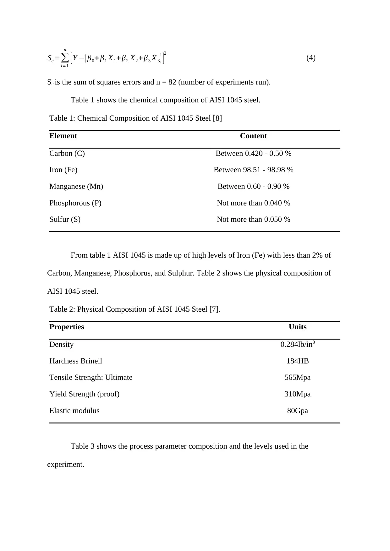
Se is the sum of squares errors and n = 82 (number of experiments run).
Table 1 shows the chemical composition of AISI 1045 steel.
Table 1: Chemical Composition of AISI 1045 Steel [8]
Element Content
Carbon (C) Between 0.420 - 0.50 %
Iron (Fe) Between 98.51 - 98.98 %
Manganese (Mn) Between 0.60 - 0.90 %
Phosphorous (P) Not more than 0.040 %
Sulfur (S) Not more than 0.050 %
From table 1 AISI 1045 is made up of high levels of Iron (Fe) with less than 2% of
Carbon, Manganese, Phosphorus, and Sulphur. Table 2 shows the physical composition of
AISI 1045 steel.
Table 2: Physical Composition of AISI 1045 Steel [7].
Properties Units
Density 0.284lb/in3
Hardness Brinell 184HB
Tensile Strength: Ultimate 565Mpa
Yield Strength (proof) 310Mpa
Elastic modulus 80Gpa
Table 3 shows the process parameter composition and the levels used in the
experiment.
i=1
n
[ Y − ( β0 + β1 X 1+ β2 X2 + β3 X 3 ) ]2
(4)
Se is the sum of squares errors and n = 82 (number of experiments run).
Table 1 shows the chemical composition of AISI 1045 steel.
Table 1: Chemical Composition of AISI 1045 Steel [8]
Element Content
Carbon (C) Between 0.420 - 0.50 %
Iron (Fe) Between 98.51 - 98.98 %
Manganese (Mn) Between 0.60 - 0.90 %
Phosphorous (P) Not more than 0.040 %
Sulfur (S) Not more than 0.050 %
From table 1 AISI 1045 is made up of high levels of Iron (Fe) with less than 2% of
Carbon, Manganese, Phosphorus, and Sulphur. Table 2 shows the physical composition of
AISI 1045 steel.
Table 2: Physical Composition of AISI 1045 Steel [7].
Properties Units
Density 0.284lb/in3
Hardness Brinell 184HB
Tensile Strength: Ultimate 565Mpa
Yield Strength (proof) 310Mpa
Elastic modulus 80Gpa
Table 3 shows the process parameter composition and the levels used in the
experiment.
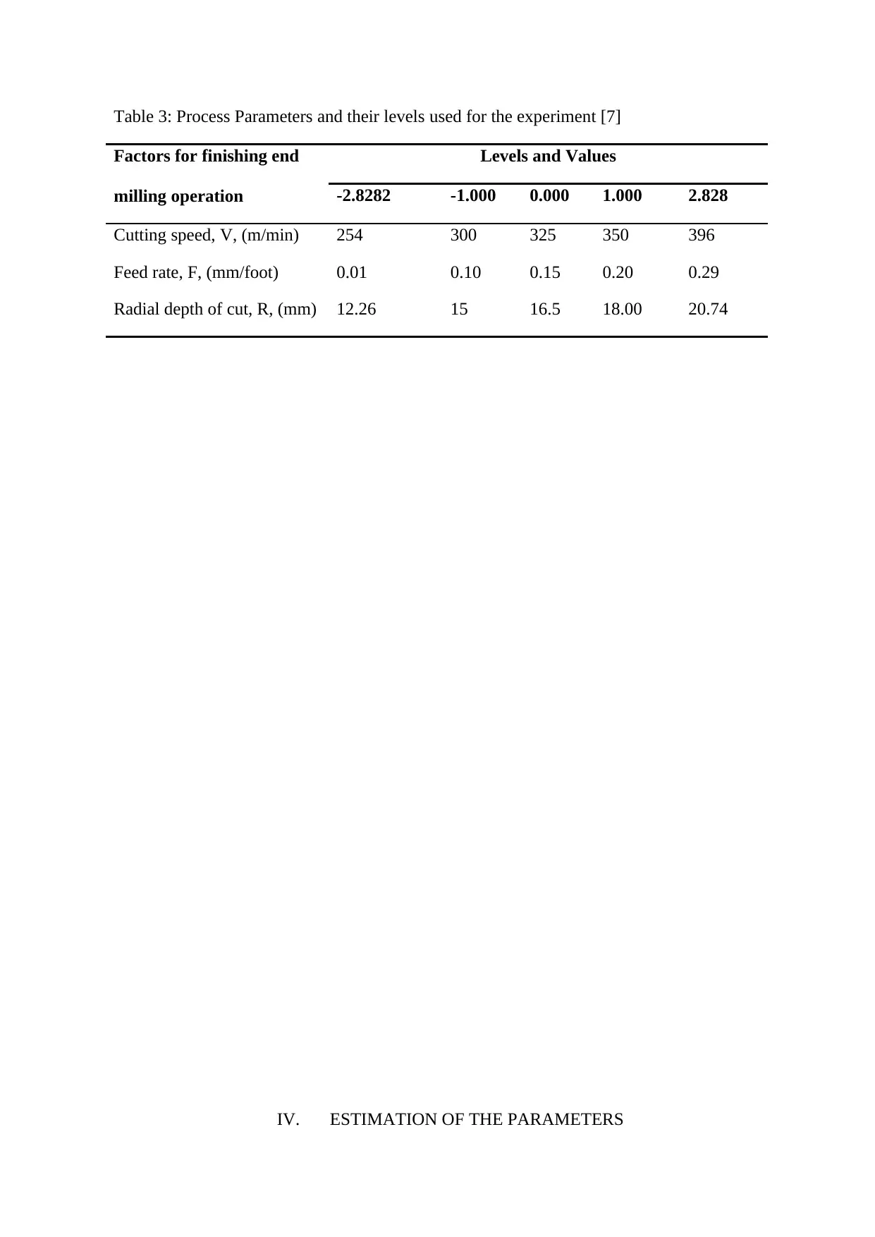
Table 3: Process Parameters and their levels used for the experiment [7]
Factors for finishing end
milling operation
Levels and Values
-2.8282 -1.000 0.000 1.000 2.828
Cutting speed, V, (m/min) 254 300 325 350 396
Feed rate, F, (mm/foot) 0.01 0.10 0.15 0.20 0.29
Radial depth of cut, R, (mm) 12.26 15 16.5 18.00 20.74
IV. ESTIMATION OF THE PARAMETERS
Factors for finishing end
milling operation
Levels and Values
-2.8282 -1.000 0.000 1.000 2.828
Cutting speed, V, (m/min) 254 300 325 350 396
Feed rate, F, (mm/foot) 0.01 0.10 0.15 0.20 0.29
Radial depth of cut, R, (mm) 12.26 15 16.5 18.00 20.74
IV. ESTIMATION OF THE PARAMETERS
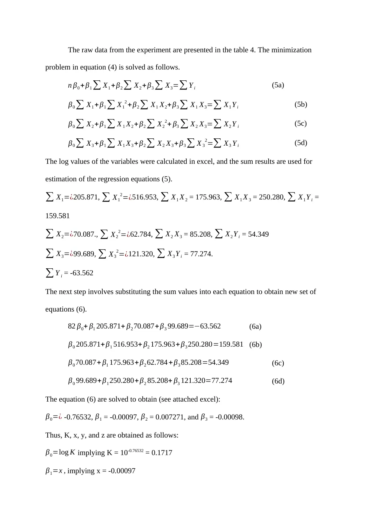
The raw data from the experiment are presented in the table 4. The minimization
problem in equation (4) is solved as follows.
n β0 + β1 ∑ X1 + β2 ∑ X2 +β3 ∑ X3=∑ Y i (5a)
β0 ∑ X1 + β1 ∑ X1
2 +β2 ∑ X1 X2+β3 ∑ X1 X3=∑ X1 Y i (5b)
β0 ∑ X2 + β1 ∑ X 1 X2 + β2 ∑ X2
2+ β3 ∑ X2 X3=∑ X2 Y i (5c)
β0 ∑ X3 + β1 ∑ X1 X3 +β2 ∑ X2 X3 + β3 ∑ X 3
2=∑ X3 Y i (5d)
The log values of the variables were calculated in excel, and the sum results are used for
estimation of the regression equations (5).
∑ X1=¿205.871, ∑ X1
2=¿516.953, ∑ X1 X 2 = 175.963, ∑ X1 X 3 = 250.280, ∑ X1 Y i =
159.581
∑ X2=¿70.087., ∑ X2
2=¿62.784, ∑ X2 X3 = 85.208, ∑ X2 Y i = 54.349
∑ X3=¿99.689, ∑ X3
2=¿121.320, ∑ X3 Y i = 77.274.
∑ Y i = -63.562
The next step involves substituting the sum values into each equation to obtain new set of
equations (6).
82 β0+ β1 205.871+ β2 70.087+ β3 99.689=−63.562 (6a)
β0 205.871+ β1 516.953+ β2 175.963+ β3 250.280=159.581 (6b)
β0 70.087+ β1 175.963+ β2 62.784 + β3 85.208=54.349 (6c)
β0 99.689+ β1 250.280+ β2 85.208+ β3 121.320=77.274 (6d)
The equation (6) are solved to obtain (see attached excel):
β0=¿ -0.76532, β1 = -0.00097, β2 = 0.007271, and β3 = -0.00098.
Thus, K, x, y, and z are obtained as follows:
β0=log K implying K = 10-0.76532 = 0.1717
β1=x , implying x = -0.00097
Paraphrase This Document
Need a fresh take? Get an instant paraphrase of this document with our AI Paraphraser
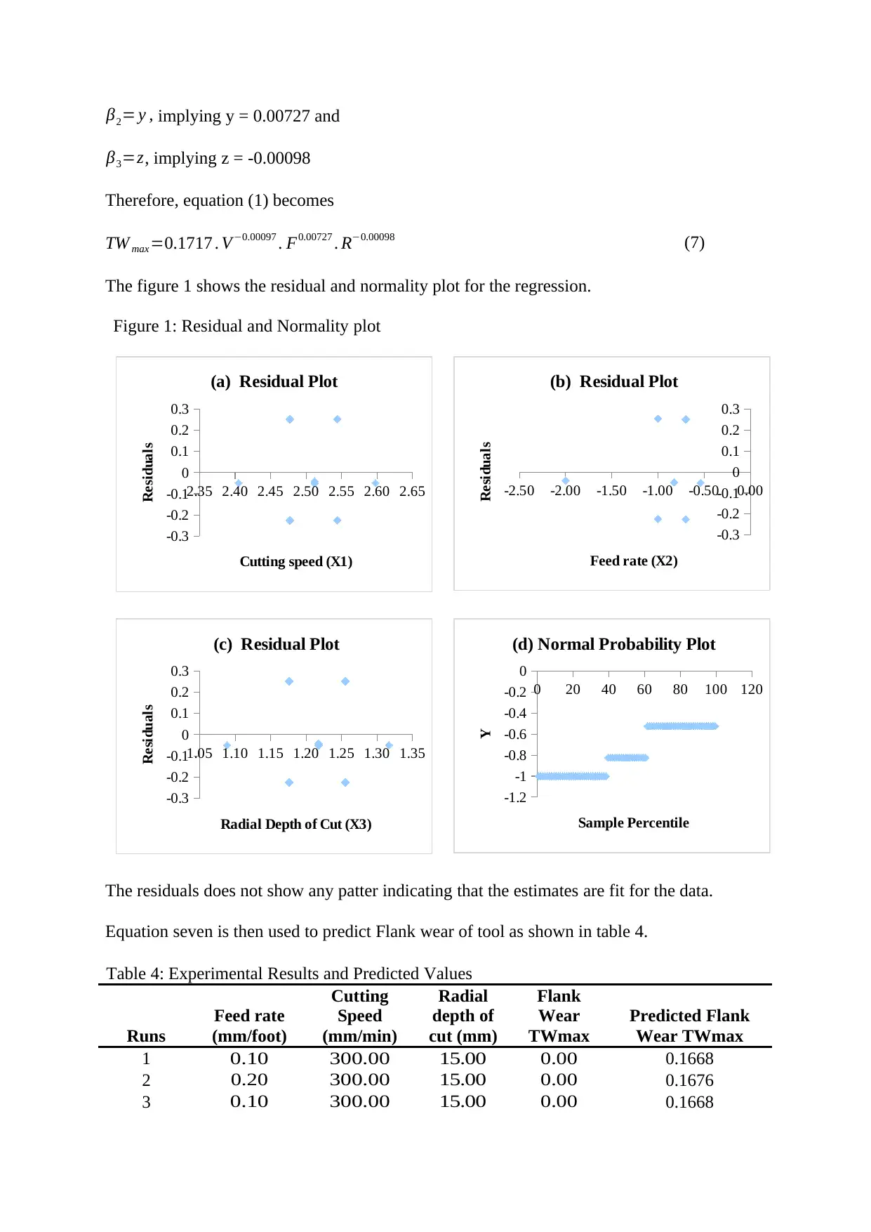
β2= y , implying y = 0.00727 and
β3=z, implying z = -0.00098
Therefore, equation (1) becomes
TW max =0.1717 . V−0.00097 . F0.00727 . R−0.00098 (7)
The figure 1 shows the residual and normality plot for the regression.
Figure 1: Residual and Normality plot
2.35 2.40 2.45 2.50 2.55 2.60 2.65
-0.3
-0.2
-0.1
0
0.1
0.2
0.3
(a) Residual Plot
Cutting speed (X1)
Residuals
-2.50 -2.00 -1.50 -1.00 -0.50 0.00
-0.3
-0.2
-0.1
0
0.1
0.2
0.3
(b) Residual Plot
Feed rate (X2)
Residuals
1.05 1.10 1.15 1.20 1.25 1.30 1.35
-0.3
-0.2
-0.1
0
0.1
0.2
0.3
(c) Residual Plot
Radial Depth of Cut (X3)
Residuals 0 20 40 60 80 100 120
-1.2
-1
-0.8
-0.6
-0.4
-0.2
0
(d) Normal Probability Plot
Sample Percentile
Y
The residuals does not show any patter indicating that the estimates are fit for the data.
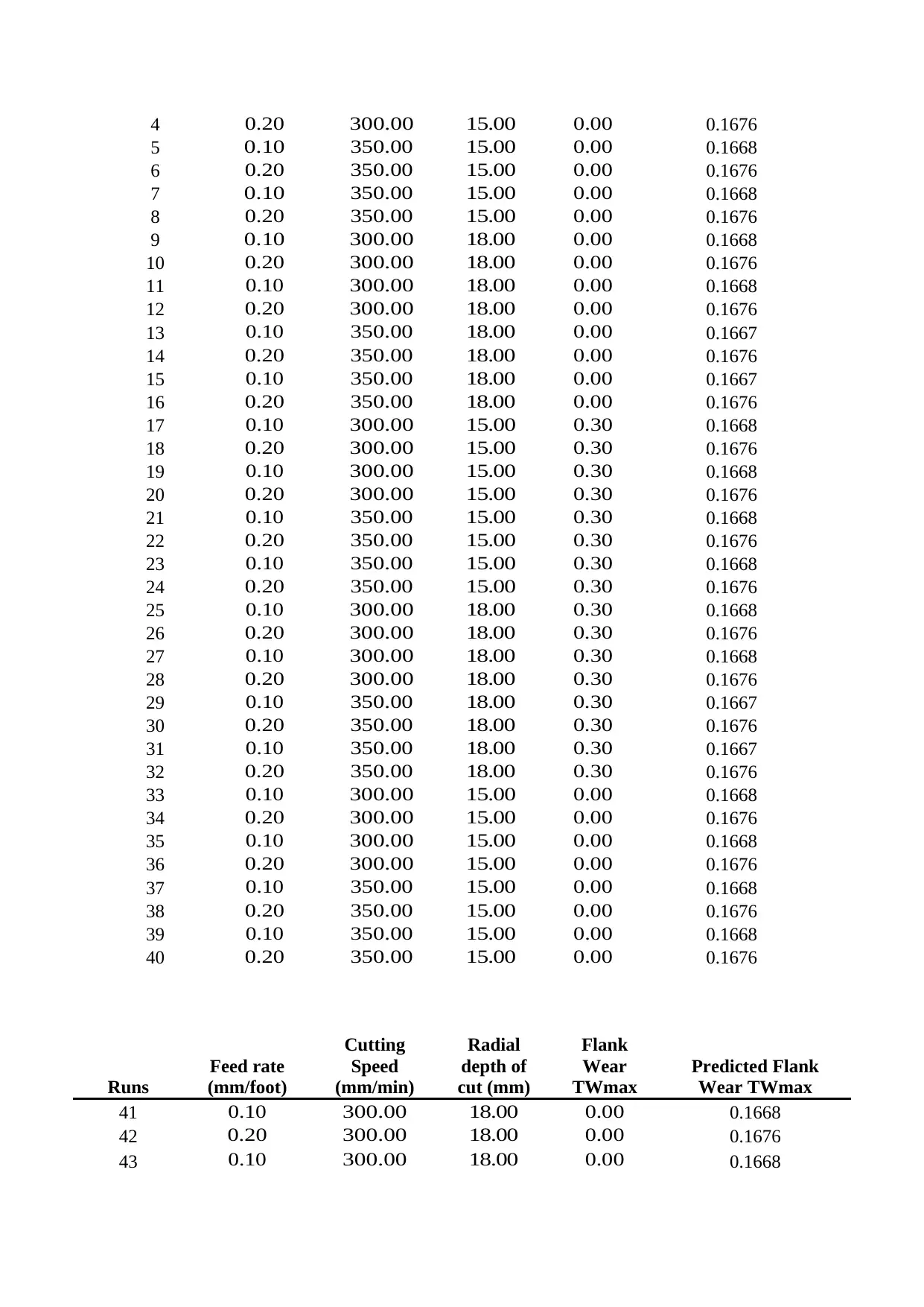
Equation seven is then used to predict Flank wear of tool as shown in table 4.
Table 4: Experimental Results and Predicted Values
Runs
Feed rate
(mm/foot)
Cutting
Speed
(mm/min)
Radial
depth of
cut (mm)
Flank
Wear
TWmax
Predicted Flank
Wear TWmax
1 0.10 300.00 15.00 0.00 0.1668
2 0.20 300.00 15.00 0.00 0.1676
3 0.10 300.00 15.00 0.00 0.1668
β3=z, implying z = -0.00098
Therefore, equation (1) becomes
TW max =0.1717 . V−0.00097 . F0.00727 . R−0.00098 (7)
The figure 1 shows the residual and normality plot for the regression.
Figure 1: Residual and Normality plot
2.35 2.40 2.45 2.50 2.55 2.60 2.65
-0.3
-0.2
-0.1
0
0.1
0.2
0.3
(a) Residual Plot
Cutting speed (X1)
Residuals
-2.50 -2.00 -1.50 -1.00 -0.50 0.00
-0.3
-0.2
-0.1
0
0.1
0.2
0.3
(b) Residual Plot
Feed rate (X2)
Residuals
1.05 1.10 1.15 1.20 1.25 1.30 1.35
-0.3
-0.2
-0.1
0
0.1
0.2
0.3
(c) Residual Plot
Radial Depth of Cut (X3)
Residuals 0 20 40 60 80 100 120
-1.2
-1
-0.8
-0.6
-0.4
-0.2
0
(d) Normal Probability Plot
Sample Percentile
Y
The residuals does not show any patter indicating that the estimates are fit for the data.
Equation seven is then used to predict Flank wear of tool as shown in table 4.
Table 4: Experimental Results and Predicted Values
Runs
Feed rate
(mm/foot)
Cutting
Speed
(mm/min)
Radial
depth of
cut (mm)
Flank
Wear
TWmax
Predicted Flank
Wear TWmax
1 0.10 300.00 15.00 0.00 0.1668
2 0.20 300.00 15.00 0.00 0.1676
3 0.10 300.00 15.00 0.00 0.1668
4 0.20 300.00 15.00 0.00 0.1676
5 0.10 350.00 15.00 0.00 0.1668
6 0.20 350.00 15.00 0.00 0.1676
7 0.10 350.00 15.00 0.00 0.1668
8 0.20 350.00 15.00 0.00 0.1676
9 0.10 300.00 18.00 0.00 0.1668
10 0.20 300.00 18.00 0.00 0.1676
11 0.10 300.00 18.00 0.00 0.1668
12 0.20 300.00 18.00 0.00 0.1676
13 0.10 350.00 18.00 0.00 0.1667
14 0.20 350.00 18.00 0.00 0.1676
15 0.10 350.00 18.00 0.00 0.1667
16 0.20 350.00 18.00 0.00 0.1676
17 0.10 300.00 15.00 0.30 0.1668
18 0.20 300.00 15.00 0.30 0.1676
19 0.10 300.00 15.00 0.30 0.1668
20 0.20 300.00 15.00 0.30 0.1676
21 0.10 350.00 15.00 0.30 0.1668
22 0.20 350.00 15.00 0.30 0.1676
23 0.10 350.00 15.00 0.30 0.1668
24 0.20 350.00 15.00 0.30 0.1676
25 0.10 300.00 18.00 0.30 0.1668
26 0.20 300.00 18.00 0.30 0.1676
27 0.10 300.00 18.00 0.30 0.1668
28 0.20 300.00 18.00 0.30 0.1676
29 0.10 350.00 18.00 0.30 0.1667
30 0.20 350.00 18.00 0.30 0.1676
31 0.10 350.00 18.00 0.30 0.1667
32 0.20 350.00 18.00 0.30 0.1676
33 0.10 300.00 15.00 0.00 0.1668
34 0.20 300.00 15.00 0.00 0.1676
35 0.10 300.00 15.00 0.00 0.1668
36 0.20 300.00 15.00 0.00 0.1676
37 0.10 350.00 15.00 0.00 0.1668
38 0.20 350.00 15.00 0.00 0.1676
39 0.10 350.00 15.00 0.00 0.1668
40 0.20 350.00 15.00 0.00 0.1676
Runs
Feed rate
(mm/foot)
Cutting
Speed
(mm/min)
Radial
depth of
cut (mm)
Flank
Wear
TWmax
Predicted Flank
Wear TWmax
41 0.10 300.00 18.00 0.00 0.1668
42 0.20 300.00 18.00 0.00 0.1676
43 0.10 300.00 18.00 0.00 0.1668
44 0.20 300.00 18.00 0.00 0.1676
45 0.10 350.00 18.00 0.00 0.1667
46 0.20 350.00 18.00 0.00 0.1676
47 0.10 350.00 18.00 0.00 0.1667
48 0.20 350.00 18.00 0.00 0.1676
49 0.10 300.00 15.00 0.30 0.1668
50 0.20 300.00 15.00 0.30 0.1676
51 0.10 300.00 15.00 0.30 0.1668
52 0.20 300.00 15.00 0.30 0.1676
53 0.10 350.00 15.00 0.30 0.1668
54 0.20 350.00 15.00 0.30 0.1676
55 0.10 350.00 15.00 0.30 0.1668
56 0.20 350.00 15.00 0.30 0.1676
57 0.10 300.00 18.00 0.30 0.1668
58 0.20 300.00 18.00 0.30 0.1676
59 0.10 300.00 18.00 0.30 0.1668
60 0.20 300.00 18.00 0.30 0.1676
61 0.10 350.00 18.00 0.30 0.1667
62 0.20 350.00 18.00 0.30 0.1676
63 0.10 350.00 18.00 0.30 0.1667
64 0.20 350.00 18.00 0.30 0.1676
65 0.01 325.00 16.50 0.15 0.1640
66 0.29 325.00 16.50 0.15 0.1681
67 0.15 325.00 16.50 0.15 0.1673
68 0.15 325.00 16.50 0.15 0.1673
69 0.15 254.00 16.50 0.15 0.1673
70 0.15 396.00 16.50 0.15 0.1672
71 0.15 325.00 12.26 0.15 0.1673
72 0.15 325.00 20.74 0.15 0.1672
73 0.15 325.00 16.50 0.15 0.1673
74 0.15 325.00 16.50 0.15 0.1673
75 0.15 325.00 16.50 0.15 0.1673
76 0.15 325.00 16.50 0.15 0.1673
77 0.15 325.00 16.50 0.15 0.1673
78 0.15 325.00 16.50 0.15 0.1673
79 0.15 325.00 16.50 0.15 0.1673
80 0.15 325.00 16.50 0.15 0.1673
81 0.15 325.00 16.50 0.15 0.1673
82 0.15 325.00 16.50 0.15 0.1673
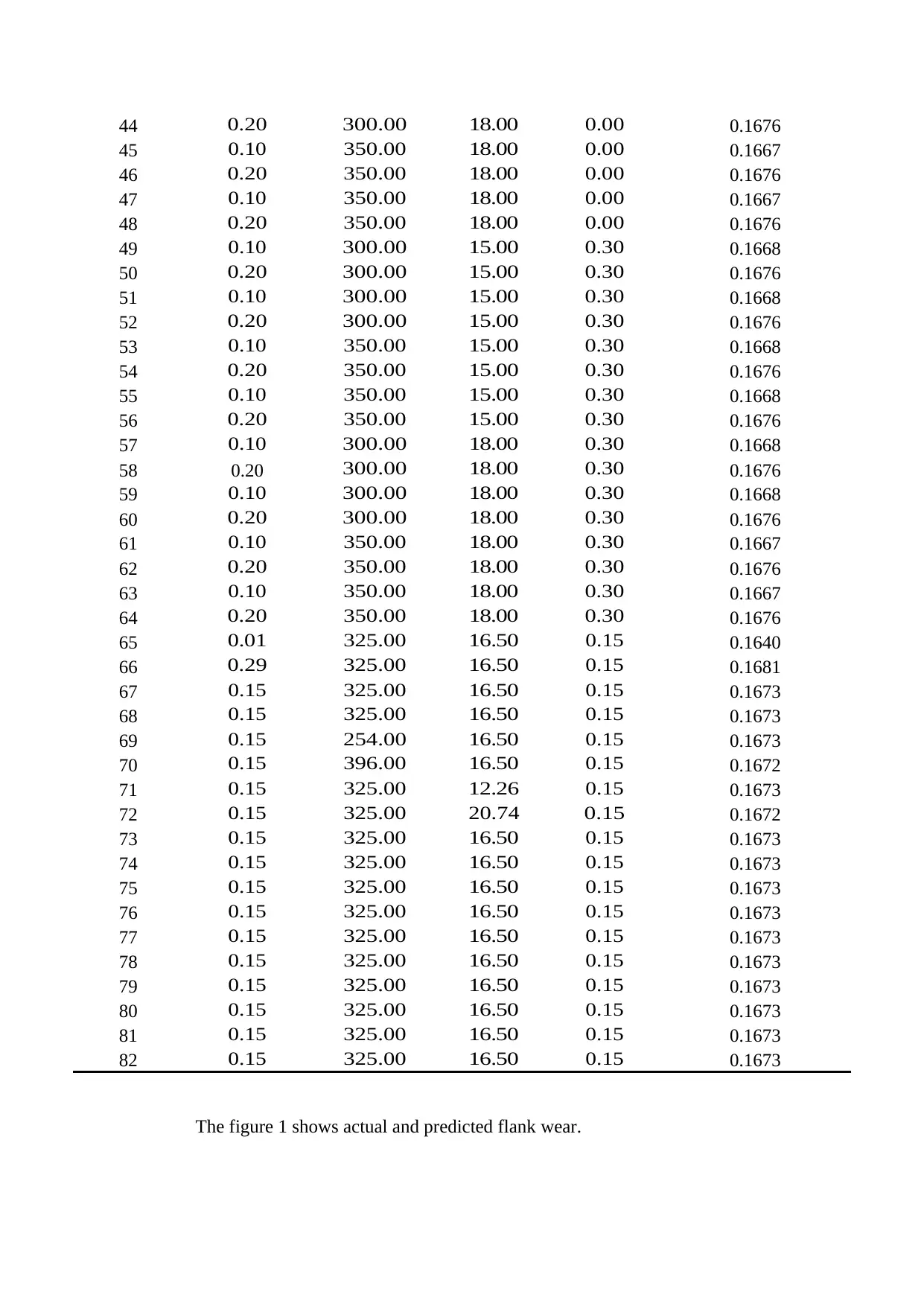
The figure 1 shows actual and predicted flank wear.
45 0.10 350.00 18.00 0.00 0.1667
46 0.20 350.00 18.00 0.00 0.1676
47 0.10 350.00 18.00 0.00 0.1667
48 0.20 350.00 18.00 0.00 0.1676
49 0.10 300.00 15.00 0.30 0.1668
50 0.20 300.00 15.00 0.30 0.1676
51 0.10 300.00 15.00 0.30 0.1668
52 0.20 300.00 15.00 0.30 0.1676
53 0.10 350.00 15.00 0.30 0.1668
54 0.20 350.00 15.00 0.30 0.1676
55 0.10 350.00 15.00 0.30 0.1668
56 0.20 350.00 15.00 0.30 0.1676
57 0.10 300.00 18.00 0.30 0.1668
58 0.20 300.00 18.00 0.30 0.1676
59 0.10 300.00 18.00 0.30 0.1668
60 0.20 300.00 18.00 0.30 0.1676
61 0.10 350.00 18.00 0.30 0.1667
62 0.20 350.00 18.00 0.30 0.1676
63 0.10 350.00 18.00 0.30 0.1667
64 0.20 350.00 18.00 0.30 0.1676
65 0.01 325.00 16.50 0.15 0.1640
66 0.29 325.00 16.50 0.15 0.1681
67 0.15 325.00 16.50 0.15 0.1673
68 0.15 325.00 16.50 0.15 0.1673
69 0.15 254.00 16.50 0.15 0.1673
70 0.15 396.00 16.50 0.15 0.1672
71 0.15 325.00 12.26 0.15 0.1673
72 0.15 325.00 20.74 0.15 0.1672
73 0.15 325.00 16.50 0.15 0.1673
74 0.15 325.00 16.50 0.15 0.1673
75 0.15 325.00 16.50 0.15 0.1673
76 0.15 325.00 16.50 0.15 0.1673
77 0.15 325.00 16.50 0.15 0.1673
78 0.15 325.00 16.50 0.15 0.1673
79 0.15 325.00 16.50 0.15 0.1673
80 0.15 325.00 16.50 0.15 0.1673
81 0.15 325.00 16.50 0.15 0.1673
82 0.15 325.00 16.50 0.15 0.1673
The figure 1 shows actual and predicted flank wear.
Secure Best Marks with AI Grader
Need help grading? Try our AI Grader for instant feedback on your assignments.
1
5
9
13
17
21
25
29
33
37
41
45
49
53
57
61
65
69
73
77
81
0.00
0.05
0.10
0.15
0.20
0.25
0.30
0.35
Figure 2: Actual and Predicted Flank Wear
Twmax Predicted Twmax
Run
Wear
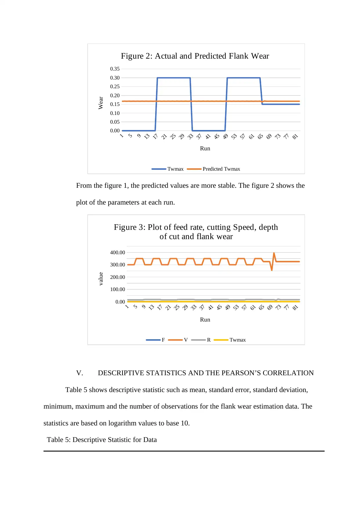
From the figure 1, the predicted values are more stable. The figure 2 shows the
plot of the parameters at each run.
1
5
9
13
17
21
25
29
33
37
41
45
49
53
57
61
65
69
73
77
81
0.00
100.00
200.00
300.00
400.00
Figure 3: Plot of feed rate, cutting Speed, depth
of cut and flank wear
F V R Twmax
Run
value
V. DESCRIPTIVE STATISTICS AND THE PEARSON’S CORRELATION
Table 5 shows descriptive statistic such as mean, standard error, standard deviation,
minimum, maximum and the number of observations for the flank wear estimation data. The
statistics are based on logarithm values to base 10.
Table 5: Descriptive Statistic for Data
5
9
13
17
21
25
29
33
37
41
45
49
53
57
61
65
69
73
77
81
0.00
0.05
0.10
0.15
0.20
0.25
0.30
0.35
Figure 2: Actual and Predicted Flank Wear
Twmax Predicted Twmax
Run
Wear
From the figure 1, the predicted values are more stable. The figure 2 shows the
plot of the parameters at each run.
1
5
9
13
17
21
25
29
33
37
41
45
49
53
57
61
65
69
73
77
81
0.00
100.00
200.00
300.00
400.00
Figure 3: Plot of feed rate, cutting Speed, depth
of cut and flank wear
F V R Twmax
Run
value
V. DESCRIPTIVE STATISTICS AND THE PEARSON’S CORRELATION
Table 5 shows descriptive statistic such as mean, standard error, standard deviation,
minimum, maximum and the number of observations for the flank wear estimation data. The
statistics are based on logarithm values to base 10.
Table 5: Descriptive Statistic for Data
Flank Wear Cutting Speed Feed rate
Radial
Depth of cut
Mean -0.78 2.51 -0.85 1.22
Standard Error 0.02 0.00 0.02 0.00
Standard
Deviation
0.21 0.03 0.19 0.04
Minimum -1.00 2.40 -2.00 1.09
Maximum -0.52 2.60 -0.54 1.32
Count 82.00 82.00 82.00 82.00
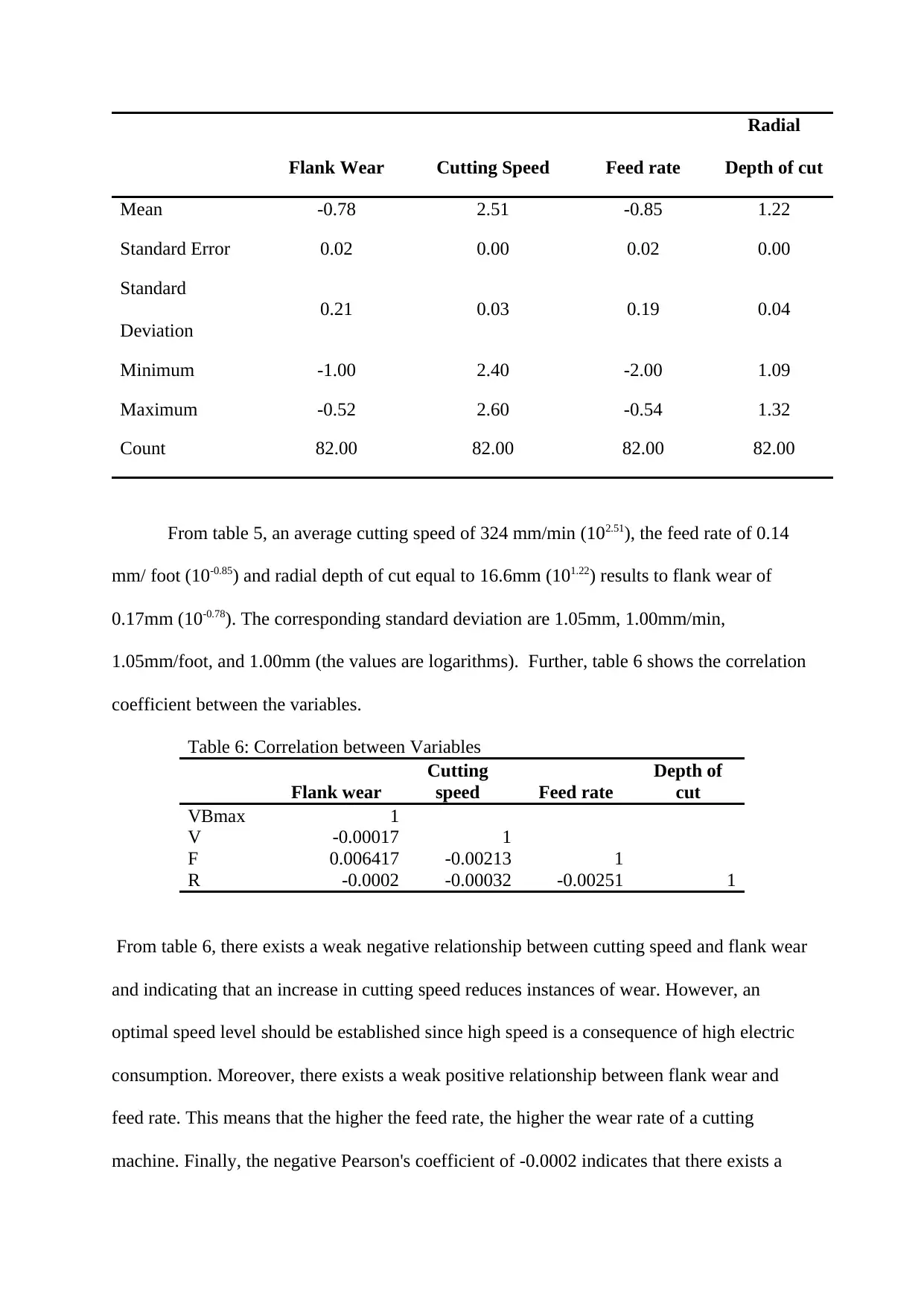
From table 5, an average cutting speed of 324 mm/min (102.51), the feed rate of 0.14
mm/ foot (10-0.85) and radial depth of cut equal to 16.6mm (101.22) results to flank wear of
0.17mm (10-0.78). The corresponding standard deviation are 1.05mm, 1.00mm/min,
1.05mm/foot, and 1.00mm (the values are logarithms). Further, table 6 shows the correlation
coefficient between the variables.
Table 6: Correlation between Variables
Flank wear
Cutting
speed Feed rate
Depth of
cut
VBmax 1
V -0.00017 1
F 0.006417 -0.00213 1
R -0.0002 -0.00032 -0.00251 1
From table 6, there exists a weak negative relationship between cutting speed and flank wear
and indicating that an increase in cutting speed reduces instances of wear. However, an
optimal speed level should be established since high speed is a consequence of high electric
consumption. Moreover, there exists a weak positive relationship between flank wear and
feed rate. This means that the higher the feed rate, the higher the wear rate of a cutting
machine. Finally, the negative Pearson's coefficient of -0.0002 indicates that there exists a
Radial
Depth of cut
Mean -0.78 2.51 -0.85 1.22
Standard Error 0.02 0.00 0.02 0.00
Standard
Deviation
0.21 0.03 0.19 0.04
Minimum -1.00 2.40 -2.00 1.09
Maximum -0.52 2.60 -0.54 1.32
Count 82.00 82.00 82.00 82.00
From table 5, an average cutting speed of 324 mm/min (102.51), the feed rate of 0.14
mm/ foot (10-0.85) and radial depth of cut equal to 16.6mm (101.22) results to flank wear of
0.17mm (10-0.78). The corresponding standard deviation are 1.05mm, 1.00mm/min,
1.05mm/foot, and 1.00mm (the values are logarithms). Further, table 6 shows the correlation
coefficient between the variables.
Table 6: Correlation between Variables
Flank wear
Cutting
speed Feed rate
Depth of
cut
VBmax 1
V -0.00017 1
F 0.006417 -0.00213 1
R -0.0002 -0.00032 -0.00251 1
From table 6, there exists a weak negative relationship between cutting speed and flank wear
and indicating that an increase in cutting speed reduces instances of wear. However, an
optimal speed level should be established since high speed is a consequence of high electric
consumption. Moreover, there exists a weak positive relationship between flank wear and
feed rate. This means that the higher the feed rate, the higher the wear rate of a cutting
machine. Finally, the negative Pearson's coefficient of -0.0002 indicates that there exists a

mild negative relationship between flank wear and radial depth of cut [2]. This indicates that
high depth results to increase in the degradation of the cutting tool.
VI. DISCUSSION AND CONCLUSION
In the operations of steel processing companies, metals cutting tools are essential and
usually accompanied by chipping, sometimes no chipping is involved [6]. In this process the
tools wear and get damaged; therefore, the paper focused in determining an equation that can
be used to predict flank wear of Cemented Carbide ISO P10 when trimming and cutting AISI
Paraphrase This Document
Need a fresh take? Get an instant paraphrase of this document with our AI Paraphraser
1045 steel. In this aspect primary data was necessary; however, an appropriate data was
obtained from a secondary source which recorded data for cutting speed, feed rate, flank wear
and radial depth of cut. The data was manipulated for averages relationships and model
building [15]. The material used for the test was AISI 1045 with an estimated hardness of
180HB. The steel was, therefore, a good representation of the actual conditions cemented
carbide ISO P10 experiences in processing companies.
Finishing end milling operations conditions usually involve significant energy
consumption, emission of heat, vibrations, and shocks. Therefore, finishing end milling is a
heavy processing condition resulting in faster tool wear or damage specifically when dealing
with steel which is hard, and tough. Thus, the estimated equation (7) can assist the
manufacturer in determining the optimal level of the three factors that cause flank wear.
However, according to Debnath, Reddy & Yi [3], cutting speed is an independent variable,
while the heat generated and the forces generated are response variables and might be
functions of numerous parameters. In this paper cutting speed is considered an independent
variable with other variables such as radial depth of cut and feed rate. There was no need of
using head generated as the response variables since the cameras used in the estimation of
flank wear provided a high level of accuracy [5].
In summary, flank wear of a material can be determined using cutting speed, feed rate
and radial depth of cut. These are predetermined parameters in any finishing or cutting
process. Therefore, machine operators can accurately determine the amount of steel that will
be cut or finished or trimmed before the tool is re-sharpened or replaced.
References
[1] Avilés, R., Albizuri, J., Rodríguez, A., & De Lacalle, L. L. (2013). Influence of low-
plasticity ball burnishing on the high-cycle fatigue strength of medium carbon AISI
1045 steel. International journal of fatigue, 55, 230-244.
[2] Bordin, A., Bruschi, S., Ghiotti, A., & Bariani, P. F. (2015). Analysis of tool wear in
cryogenic machining of additive manufactured Ti6Al4V alloy. Wear, 328, 89-99.
[3] Debnath, S., Reddy, M. M., & Yi, Q. S. (2016). Influence of cutting fluid conditions
and cutting parameters on surface roughness and tool wear in turning process using
Taguchi method. Measurement, 78, 111-119.
[4] Fayomi, O. S. I. (2018). Data on the optimized sulphate electrolyte zinc rich coating
produced through in-situ variation of process parameters. Data in brief, 16, 141-146.
[5] Krolczyk, G. M., Nieslony, P., & Legutko, S. (2015). Determination of tool life and
research wear during duplex stainless steel turning. Archives of Civil and Mechanical
Engineering, 15(2), 347-354.
[6] Kümmel, J., Braun, D., Gibmeier, J., Schneider, J., Greiner, C., Schulze, V., &
Wanner, A. (2015). Study on micro texturing of uncoated cemented carbide cutting
tools for wear improvement and built-up edge stabilisation. Journal of Materials
Processing Technology, 215, 62-70.
[7] Lopes, L. G. D., de Brito, T. G., de Paiva, A. P., Peruchi, R. S., & Balestrassi, P. P.
(2016). Experimental design and data collection of a finishing end milling operation
of AISI 1045 steel. Data Brief, 6, 609-613.
[8] Nwoke, O. N., Okonkwo, U. C., Okafor, C. E., & Okokpujie, I. P. (2017). Evaluation
of Chatter Vibration Frequency In Cnc Turning of 4340 Alloy Steel
Material. International Journal of Scientific & Engineering Research, 8(2), 487-495.
[9] Okokpujie, I. P, Okonkwo, U.C. (2015). Effects of cutting parameters on surface
roughness during end milling of aluminium under minimum quantity lubrication
(MQL). Int. J. Sci. Res., 4(5), 2937-2942.
[10] Okokpujie, I., Okonkwo, U., & Okwudibe, C. (2015). Cutting parameters
effects on surface roughness during end milling of aluminium 6061 alloy under dry
machining operation. International Journal of Science and Research, 4(7), 2030-
2036.
Secure Best Marks with AI Grader
Need help grading? Try our AI Grader for instant feedback on your assignments.
[11] Okokpujie, I.J, Ikumapayi, O.M., Okonkwo, U.C., Salawu, E.Y., Afolalu,
S.A., Dirisu, J.O., ... & Ajayi, O.O., (2017). Experimental and Mathematical
Modeling for Prediction of Tool Wear on the Machining of Aluminium 6061 Alloy by
High Speed Steel Tools. Open Engineering., 7(1), 461–469.
[12] Okonkwo, U. C., Okokpujie, I. P., Sinebe, J. E., & Ezugwu, C. A. (2015).
Comparative analysis of aluminium surface roughness in end-milling under dry and
minimum quantity lubrication (MQL) conditions. Manufacturing Review, 2(30), 1-11.
[13] Ramesh, S., Karunamoorthy, L., & Palanikumar, K. (2008). Fuzzy modeling
and analysis of machining parameters in machining titanium alloy. Materials and
Manufacturing Processes, 23(4), 439-447.
[14] Rivero, A., Aramendi, G., Herranz, S., & de Lacalle, L. L. (2006). An
experimental investigation of the effect of coatings and cutting parameters on the dry
drilling performance of aluminium alloys. The International Journal of Advanced
Manufacturing Technology, 28(1-2), 1-11.
[15] Selvaraj, D. P., & Chandramohan, P. (2010). Optimization of surface
roughness of AISI 304 austenitic stainless steel in dry turning operation using Taguchi
design method. Journal of engineering science and technology, 5(3), 293-301.
[16] Okokpujie, I. P., Ohunakin, O. S., Bolu, C. A., & Okokpujie, K. O. (2018).
Experimental data-set for prediction of tool wear during turning of Al-1061 alloy by
high speed steel cutting tools. Data in brief, 18, 1196-1203.
1 out of 17
Your All-in-One AI-Powered Toolkit for Academic Success.
+13062052269
info@desklib.com
Available 24*7 on WhatsApp / Email
![[object Object]](/_next/static/media/star-bottom.7253800d.svg)
Unlock your academic potential
© 2024 | Zucol Services PVT LTD | All rights reserved.