Solved Probability and Statistics Assignment: Comprehensive Solution

This assignment solution covers fundamental concepts in probability and statistics, including the definition and measurement of probability, the concept of statistical independence, and calculations involving probability distributions. It includes an analysis of daily sales data using Excel to determine e...Read More

Probability statistics 1
Probability statistics
Student name:
Tutor name:

Probability statistics 2
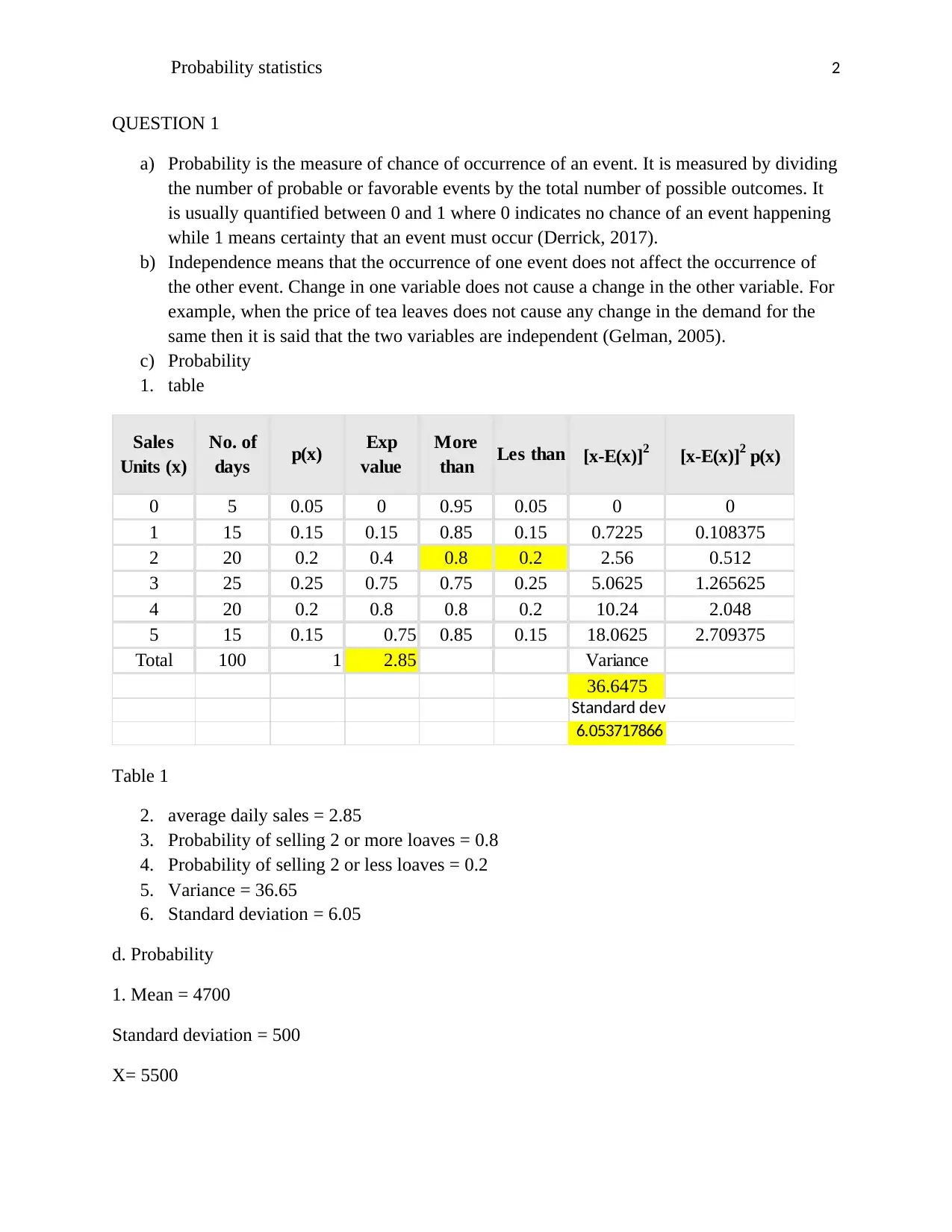
QUESTION 1
a) Probability is the measure of chance of occurrence of an event. It is measured by dividing
the number of probable or favorable events by the total number of possible outcomes. It
is usually quantified between 0 and 1 where 0 indicates no chance of an event happening
while 1 means certainty that an event must occur (Derrick, 2017).
b) Independence means that the occurrence of one event does not affect the occurrence of
the other event. Change in one variable does not cause a change in the other variable. For
example, when the price of tea leaves does not cause any change in the demand for the
same then it is said that the two variables are independent (Gelman, 2005).
c) Probability
1. table
Sales
Units (x)
No. of
days p(x) Exp
value
More
than Les than [x-E(x)]2 [x-E(x)]2 p(x)
0 5 0.05 0 0.95 0.05 0 0
1 15 0.15 0.15 0.85 0.15 0.7225 0.108375
2 20 0.2 0.4 0.8 0.2 2.56 0.512
3 25 0.25 0.75 0.75 0.25 5.0625 1.265625
4 20 0.2 0.8 0.8 0.2 10.24 2.048
5 15 0.15 0.75 0.85 0.15 18.0625 2.709375
Total 100 1 2.85 Variance
36.6475
Standard dev
6.053717866
Table 1
2. average daily sales = 2.85
3. Probability of selling 2 or more loaves = 0.8
4. Probability of selling 2 or less loaves = 0.2
5. Variance = 36.65
6. Standard deviation = 6.05
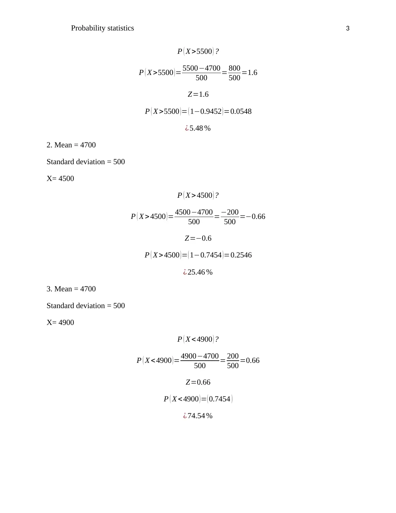
d. Probability
1. Mean = 4700
Standard deviation = 500
X= 5500

Probability statistics 3
P ( X >5500 ) ?
P ( X >5500 )= 5500−4700
500 = 800
500 =1.6
Z=1.6
P ( X >5500 )= ( 1−0.9452 )=0.0548
¿ 5.48 %
2. Mean = 4700
Standard deviation = 500
X= 4500
P ( X > 4500 ) ?
P ( X > 4500 ) = 4500−4700
500 =−200
500 =−0.66
Z=−0.6
P ( X > 4500 ) = ( 1−0.7454 ) =0.2546
¿ 25.46 %
3. Mean = 4700
Standard deviation = 500
X= 4900
P ( X < 4900 ) ?
P ( X < 4900 ) = 4900−4700
500 = 200
500 =0.66
Z=0.66
P ( X < 4900 )= ( 0.7454 )
¿ 74.54 %

Probability statistics 4
4. Mean = 4700
Standard deviation = 500
X= 4300
P ( X < 4300 ) ?
P ( X < 4300 )= 4300−4700
500 =−400
500 =−0.8
Z=−0.8
P ( X < 4300 ) = ( 1−0.7881 ) =0.2119
¿ 21.19 %
QUESTION 2
1.
Worksheet 1
Australia's population pyramid
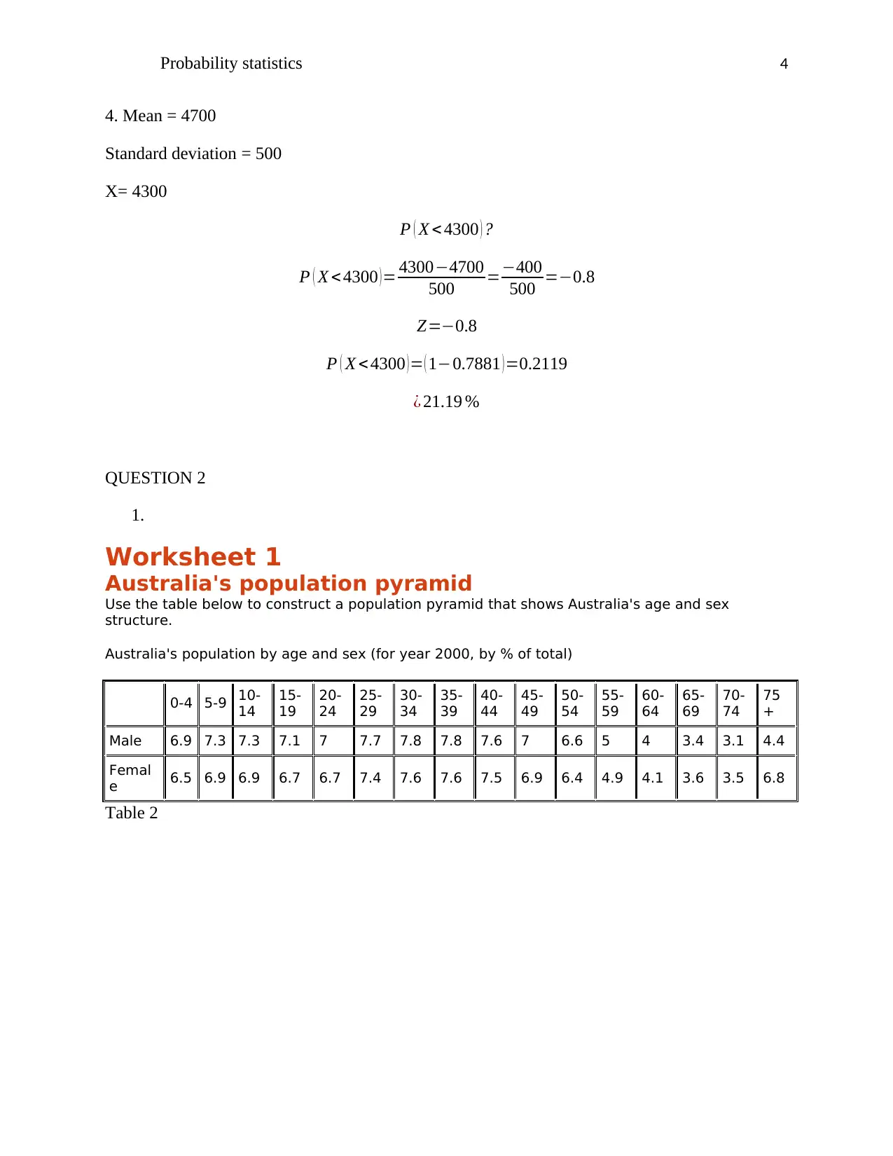
Use the table below to construct a population pyramid that shows Australia's age and sex
structure.
Australia's population by age and sex (for year 2000, by % of total)
0-4 5-9 10-
14
15-
19
20-
24
25-
29
30-
34
35-
39
40-
44
45-
49
50-
54
55-
59
60-
64
65-
69
70-
74
75
+
Male 6.9 7.3 7.3 7.1 7 7.7 7.8 7.8 7.6 7 6.6 5 4 3.4 3.1 4.4
Femal
e 6.5 6.9 6.9 6.7 6.7 7.4 7.6 7.6 7.5 6.9 6.4 4.9 4.1 3.6 3.5 6.8
Table 2

Probability statistics 5
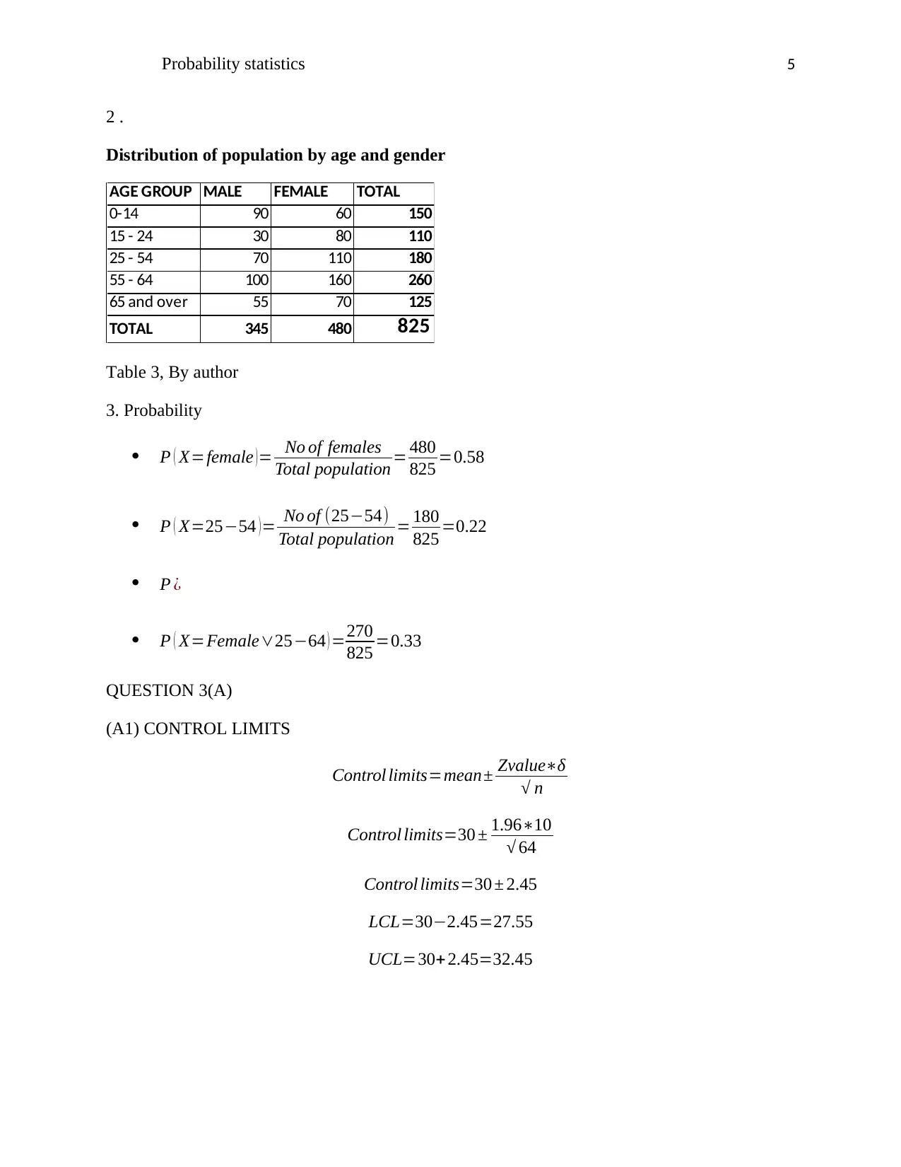
2 .
Distribution of population by age and gender
AGE GROUP MALE FEMALE TOTAL
0-14 90 60 150
15 - 24 30 80 110
25 - 54 70 110 180
55 - 64 100 160 260
65 and over 55 70 125
TOTAL 345 480 825
Table 3, By author
3. Probability
 P ( X=female )= No of females
Total population = 480
825 =0.58
 P ( X=25−54 )= No of (25−54)
Total population = 180
825 =0.22
 P ¿
 P ( X=Female∨25−64 ) =270
825 =0.33
QUESTION 3(A)
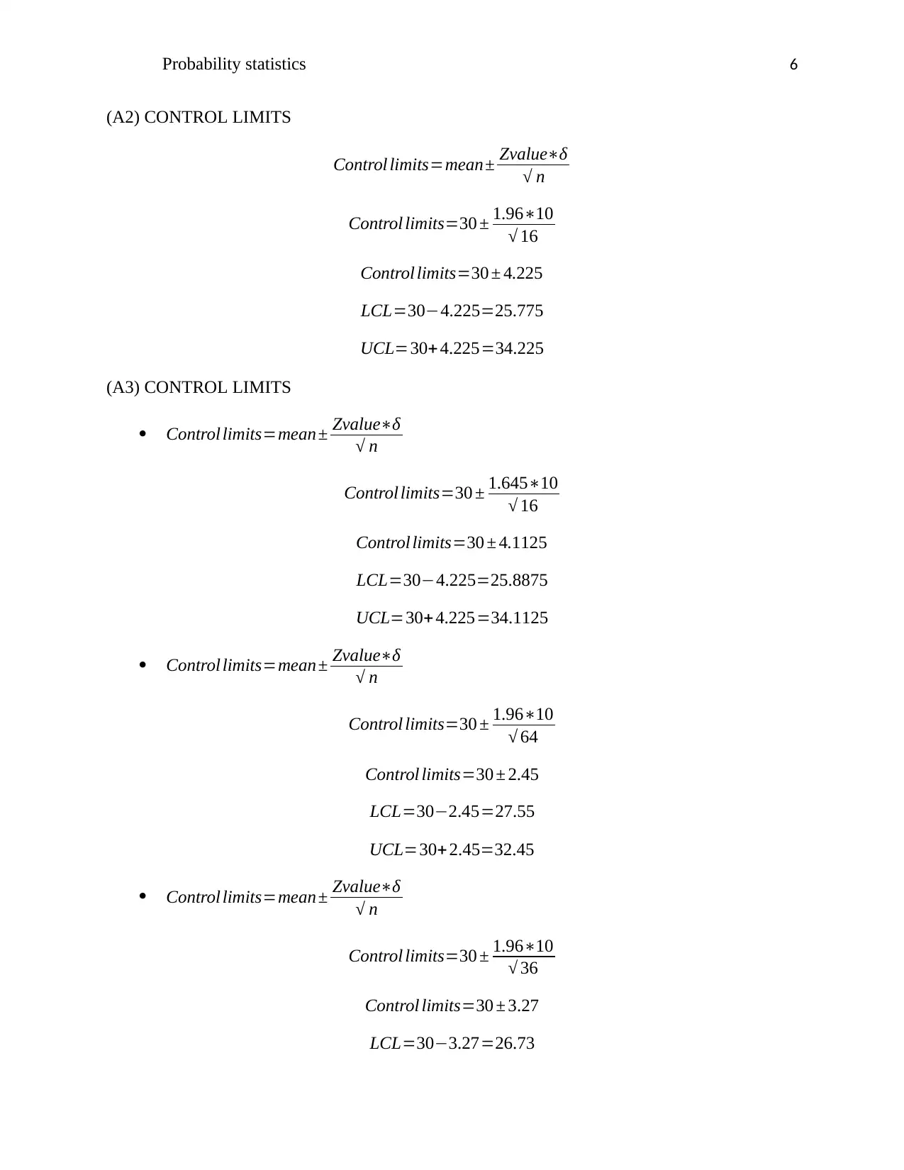
(A1) CONTROL LIMITS
Control limits=mean± Zvalue∗δ
√ n
Control limits=30 ± 1.96∗10
√ 64
Control limits=30 ± 2.45
LCL=30−2.45=27.55
UCL=30+ 2.45=32.45

Probability statistics 6
(A2) CONTROL LIMITS
Control limits=mean± Zvalue∗δ
√ n
Control limits=30 ± 1.96∗10
√ 16
Control limits=30 ± 4.225
LCL=30−4.225=25.775
UCL=30+ 4.225=34.225
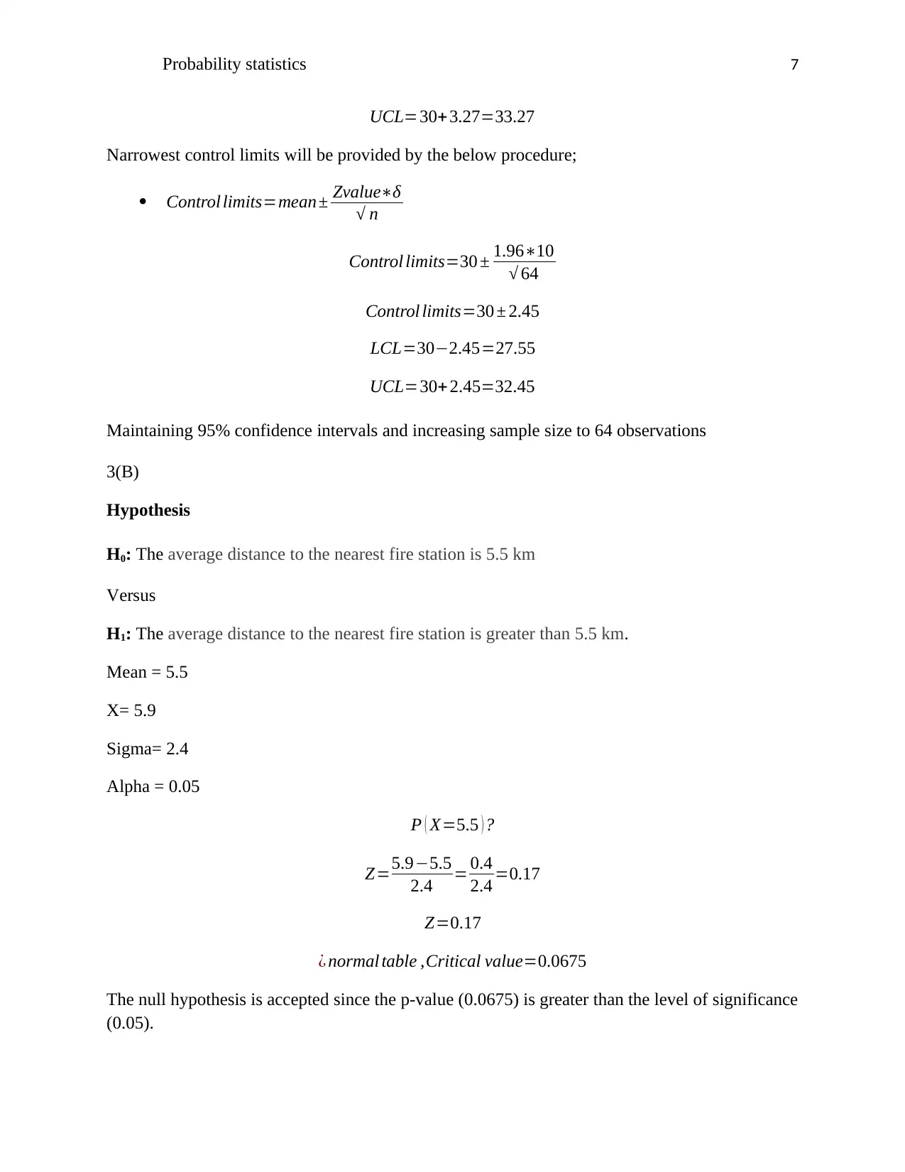
(A3) CONTROL LIMITS
 Control limits=mean± Zvalue∗δ
√ n
Control limits=30 ± 1.645∗10
√ 16
Control limits=30 ± 4.1125
LCL=30−4.225=25.8875
UCL=30+ 4.225=34.1125
 Control limits=mean± Zvalue∗δ
√ n
Control limits=30 ± 1.96∗10
√ 64
Control limits=30 ± 2.45
LCL=30−2.45=27.55
UCL=30+ 2.45=32.45
 Control limits=mean± Zvalue∗δ
√ n
Control limits=30 ± 1.96∗10
√ 36
Control limits=30 ± 3.27
LCL=30−3.27=26.73

Probability statistics 7
UCL=30+3.27=33.27
Narrowest control limits will be provided by the below procedure;
 Control limits=mean± Zvalue∗δ
√ n
Control limits=30 ± 1.96∗10
√ 64
Control limits=30 ± 2.45
LCL=30−2.45=27.55
UCL=30+ 2.45=32.45
Maintaining 95% confidence intervals and increasing sample size to 64 observations
3(B)
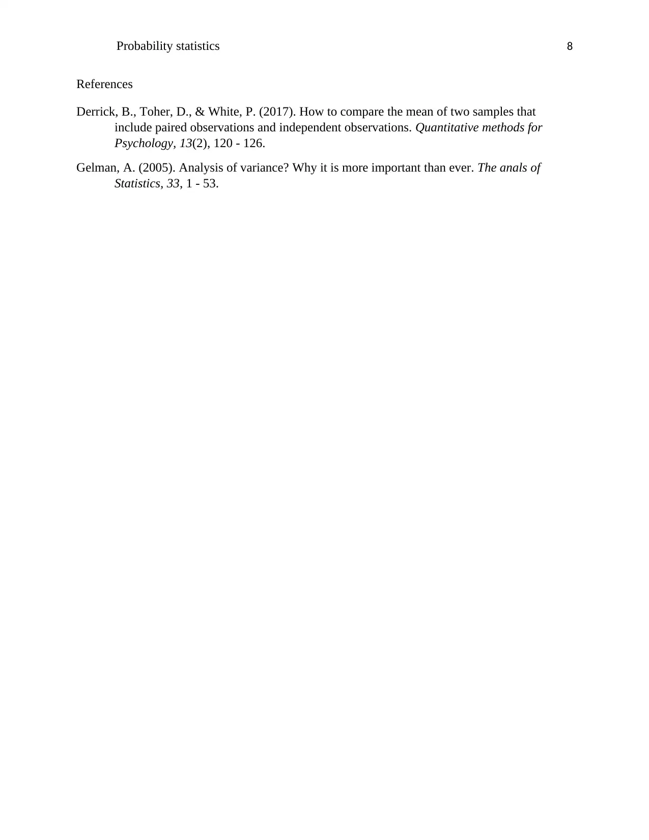
Hypothesis
H0: The average distance to the nearest fire station is 5.5 km
Versus
H1: The average distance to the nearest fire station is greater than 5.5 km.
Mean = 5.5
X= 5.9
Sigma= 2.4
Alpha = 0.05
P ( X=5.5 ) ?
Z=5.9−5.5
2.4 = 0.4
2.4 =0.17
Z=0.17
¿ normal table ,Critical value=0.0675
The null hypothesis is accepted since the p-value (0.0675) is greater than the level of significance
(0.05).

Probability statistics 8
References
Derrick, B., Toher, D., & White, P. (2017). How to compare the mean of two samples that
include paired observations and independent observations. Quantitative methods for
Psychology, 13(2), 120 - 126.
Gelman, A. (2005). Analysis of variance? Why it is more important than ever. The anals of
Statistics, 33, 1 - 53.