Problem Sheet 5

Running head: PROBLEM SHEET 5 1
Problem Sheet 5
Name
Institution

PROBLEM SHEET 5 2
Part a
Gain , k=2
Time Constant ,T =30 μs
G(s)= k
1+Ts = 2
1+30 ×10−6 s
Applying the frequency response theorem to the above equation yields:
G ( jω ) = K
1+ω2 T 2 − j ωKT
1+ω2 T 2 = 2
1+ω2 ( 30 ×10−6 ) 2 − j ω(2 ×30 ×10−6)
1+ ω2 ( 30× 10−6 ) 2
¿ 2
1+ 9× 10−10 ω2 − j 6 ×10−5 ω
1+ 9 ×10−10 ω2
|G ( jω )|= K
√1+ω2 T 2 = 2
√1+9 ×10−10 ω2 =20 log 2
√1+ 9 ×10−10 ω2 decibels
arg ( G ( jω ) )=tan−1 {−30 ×10−6 ω }= 180
π tan−1 {−30 ×10−6 ω } degrees
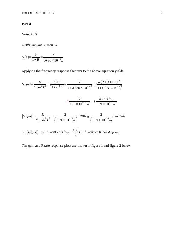
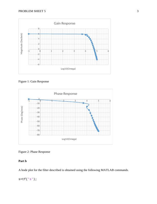
The gain and Phase response plots are shown in figure 1 and figure 2 below.

PROBLEM SHEET 5 3
-1 0 1 2 3 4 5 6
-6
-4
-2
0
2
4
6
8
Gain Response
Log10(Omega)
Magnitude (Decibels)
Figure 1: Gain Response
-1 0 1 2 3 4 5 6
-80
-70
-60
-50
-40
-30
-20
-10
0
Phase Response
Log10(Omega)
Phase (Deg)rees)
Figure 2: Phase Response
Part b
A bode plot for the filter described is obtained using the following MATLAB commands.
s=tf('s');