Problems of Statistics - Desklib

This article discusses problems of statistics including frequency distribution, cumulative frequency distribution, relative frequency distribution, cumulative relative frequency distribution, ANOVA, and regression analysis. It also includes tables and figures to support the explanations.

6
Problems of Statistics

6
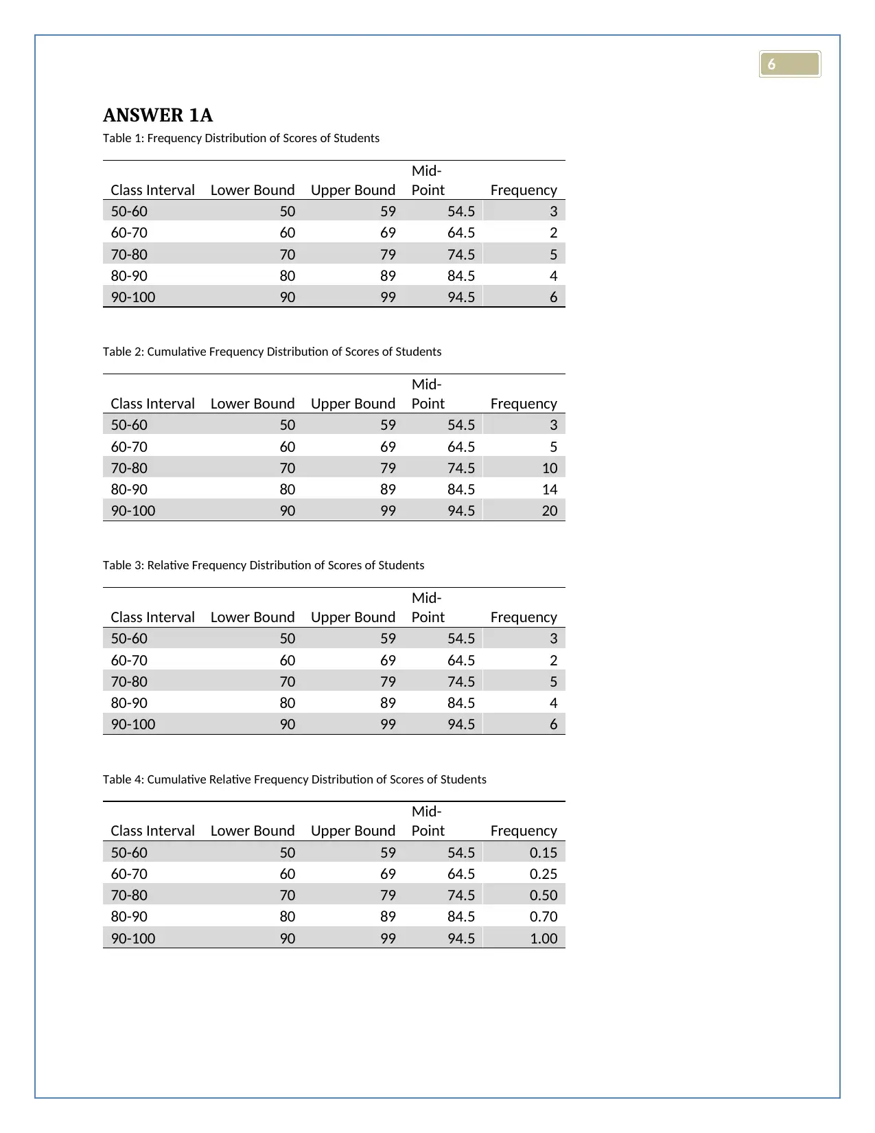
ANSWER 1A
Table 1: Frequency Distribution of Scores of Students
Class Interval Lower Bound Upper Bound
Mid-
Point Frequency
50-60 50 59 54.5 3
60-70 60 69 64.5 2
70-80 70 79 74.5 5
80-90 80 89 84.5 4
90-100 90 99 94.5 6
Table 2: Cumulative Frequency Distribution of Scores of Students
Class Interval Lower Bound Upper Bound
Mid-
Point Frequency
50-60 50 59 54.5 3
60-70 60 69 64.5 5
70-80 70 79 74.5 10
80-90 80 89 84.5 14
90-100 90 99 94.5 20
Table 3: Relative Frequency Distribution of Scores of Students
Class Interval Lower Bound Upper Bound
Mid-
Point Frequency
50-60 50 59 54.5 3
60-70 60 69 64.5 2
70-80 70 79 74.5 5
80-90 80 89 84.5 4
90-100 90 99 94.5 6
Table 4: Cumulative Relative Frequency Distribution of Scores of Students
Class Interval Lower Bound Upper Bound
Mid-
Point Frequency
50-60 50 59 54.5 0.15
60-70 60 69 64.5 0.25
70-80 70 79 74.5 0.50
80-90 80 89 84.5 0.70
90-100 90 99 94.5 1.00

6
Table 5: Percent Frequency Distribution of Scores of Students
Class Interval Lower Bound Upper Bound
Mid-
Point Frequency
50-60 50 59 54.5 15.00%
60-70 60 69 64.5 10.00%
70-80 70 79 74.5 25.00%
80-90 80 89 84.5 20.00%
90-100 90 99 94.5 30.00%
ANSWER 1B
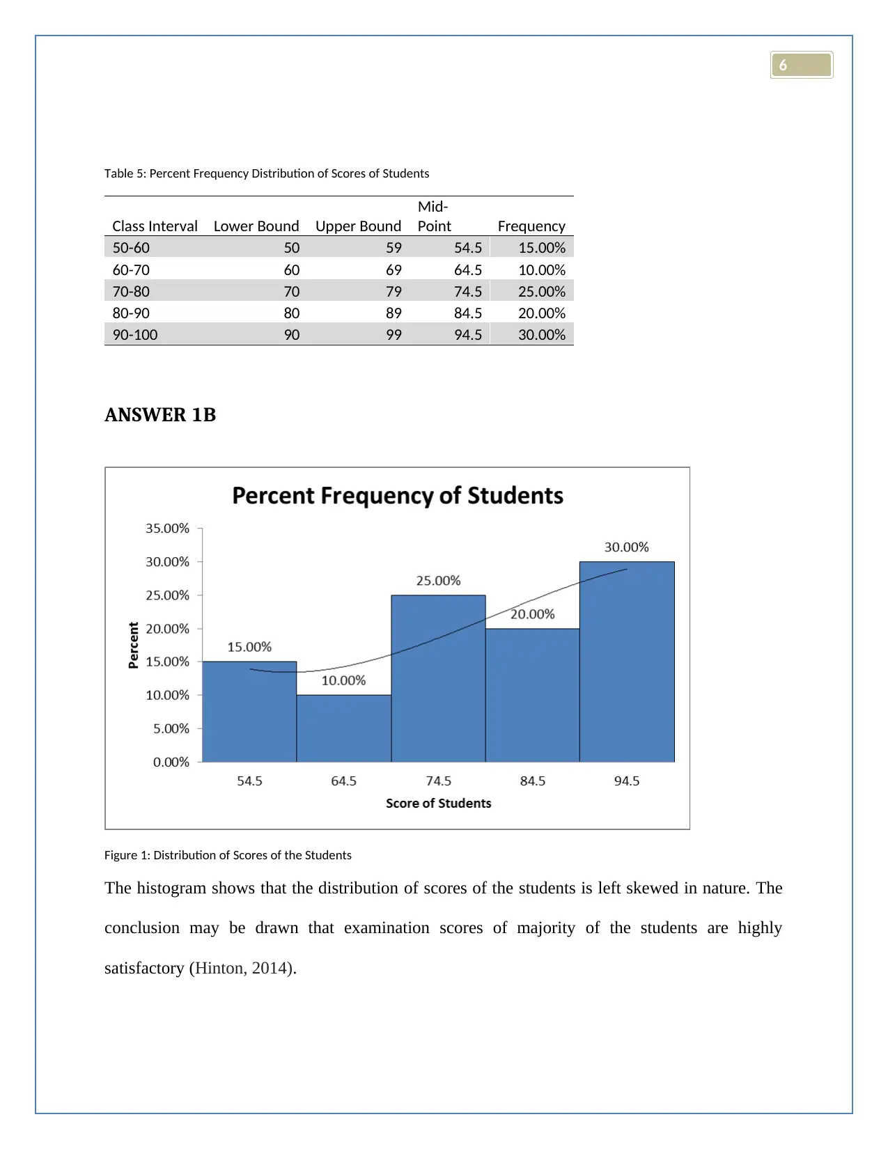
Figure 1: Distribution of Scores of the Students
The histogram shows that the distribution of scores of the students is left skewed in nature. The
conclusion may be drawn that examination scores of majority of the students are highly
satisfactory (Hinton, 2014).

6
ANSWER 2 A
The degree of freedom for residual is always sample size minus two. Hence sample size is
(39+2) = 41 for the current problem.
ANSWER 2 B
Standard error of unit price indicated that about 95% of the data should belong within 2*standard
error (SE) of the estimate. For the current problem, it is observed that about 95% of the data falls
within 0.042% of the fitted line of regression model. Hence, supply (demand) has a strong linear
relation with unit price with low gradient.
ANSWER 2 C
From the regression model SSM (sum square model) =354.689, SSE (sum square error) =
7035.262, hence, SST (sum square total) = SSE + SSM = 354.689 +7035.262 = 7389.951.
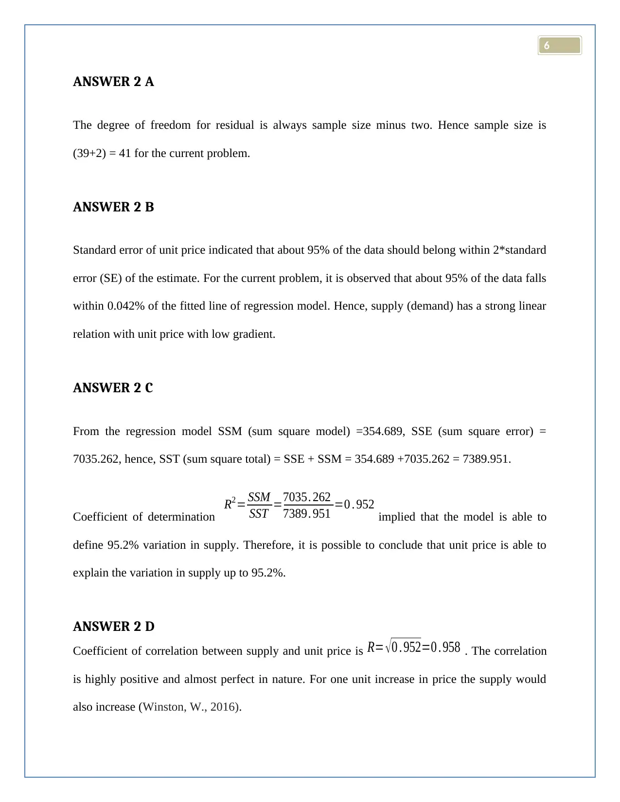
Coefficient of determination
R2= SSM
SST =7035. 262
7389. 951 =0 . 952 implied that the model is able to
define 95.2% variation in supply. Therefore, it is possible to conclude that unit price is able to
explain the variation in supply up to 95.2%.
ANSWER 2 D
Coefficient of correlation between supply and unit price is R= √ 0 . 952=0 . 958 . The correlation
is highly positive and almost perfect in nature. For one unit increase in price the supply would
also increase (Winston, W., 2016).

6
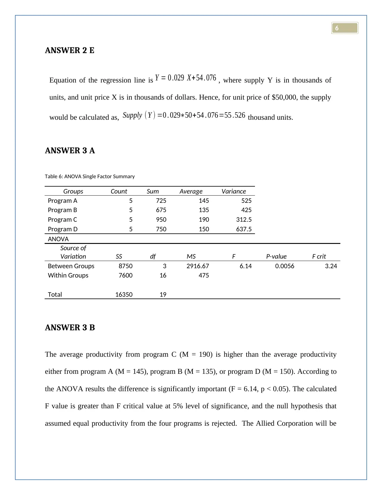
ANSWER 2 E
Equation of the regression line is Y = 0 .029 X+ 54 . 076 , where supply Y is in thousands of
units, and unit price X is in thousands of dollars. Hence, for unit price of $50,000, the supply
would be calculated as, Supply ( Y ) =0 . 029∗50+54 . 076=55 .526 thousand units.
ANSWER 3 A
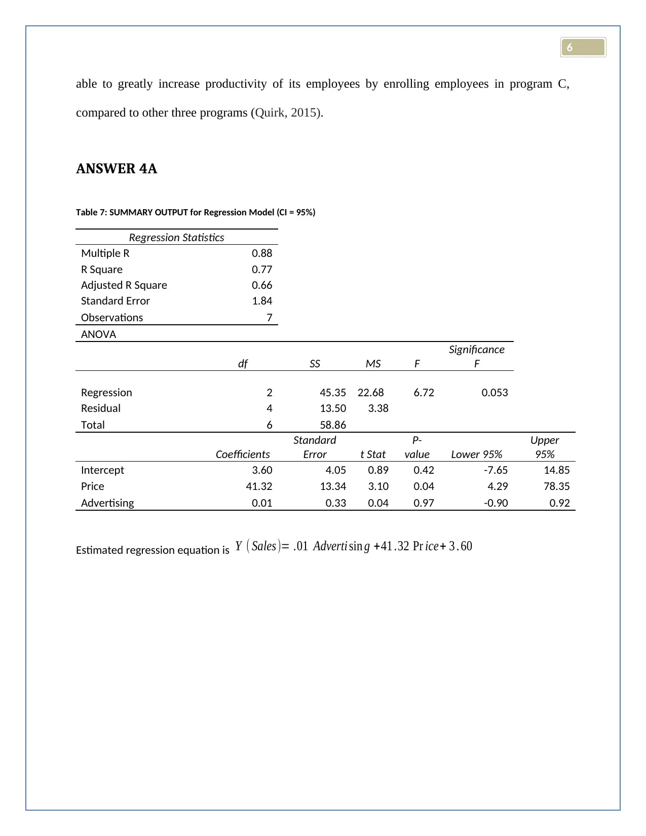
Table 6: ANOVA Single Factor Summary
Groups Count Sum Average Variance
Program A 5 725 145 525
Program B 5 675 135 425
Program C 5 950 190 312.5
Program D 5 750 150 637.5
ANOVA
Source of
Variation SS df MS F P-value F crit
Between Groups 8750 3 2916.67 6.14 0.0056 3.24
Within Groups 7600 16 475
Total 16350 19
ANSWER 3 B
The average productivity from program C (M = 190) is higher than the average productivity
either from program A (M = 145), program B (M = 135), or program D (M = 150). According to
the ANOVA results the difference is significantly important (F = 6.14, p < 0.05). The calculated
F value is greater than F critical value at 5% level of significance, and the null hypothesis that
assumed equal productivity from the four programs is rejected. The Allied Corporation will be

6
able to greatly increase productivity of its employees by enrolling employees in program C,
compared to other three programs (Quirk, 2015).
ANSWER 4A
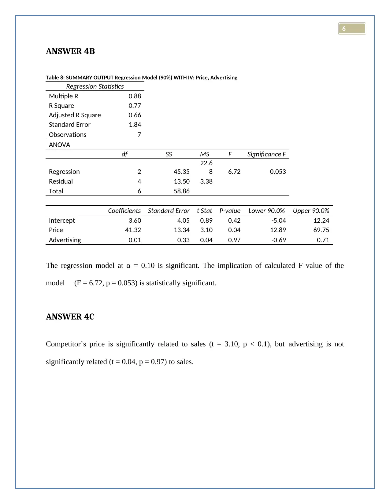
Table 7: SUMMARY OUTPUT for Regression Model (CI = 95%)
Regression Statistics
Multiple R 0.88
R Square 0.77
Adjusted R Square 0.66
Standard Error 1.84
Observations 7
ANOVA
df SS MS F
Significance
F
Regression 2 45.35 22.68 6.72 0.053
Residual 4 13.50 3.38
Total 6 58.86
Coefficients
Standard
Error t Stat
P-
value Lower 95%
Upper
95%
Intercept 3.60 4.05 0.89 0.42 -7.65 14.85
Price 41.32 13.34 3.10 0.04 4.29 78.35
Advertising 0.01 0.33 0.04 0.97 -0.90 0.92
Estimated regression equation is Y ( Sales)= .01 Adverti sin g +41 .32 Pr ice+ 3 . 60

6
ANSWER 4B
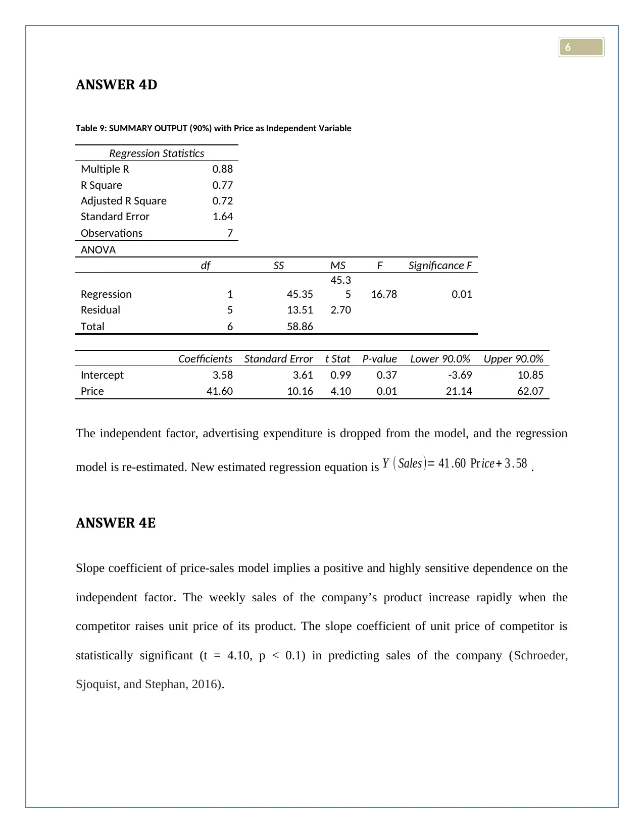
Table 8: SUMMARY OUTPUT Regression Model (90%) WITH IV: Price, Advertising
Regression Statistics
Multiple R 0.88
R Square 0.77
Adjusted R Square 0.66
Standard Error 1.84
Observations 7
ANOVA
df SS MS F Significance F
Regression 2 45.35
22.6
8 6.72 0.053
Residual 4 13.50 3.38
Total 6 58.86
Coefficients Standard Error t Stat P-value Lower 90.0% Upper 90.0%
Intercept 3.60 4.05 0.89 0.42 -5.04 12.24
Price 41.32 13.34 3.10 0.04 12.89 69.75
Advertising 0.01 0.33 0.04 0.97 -0.69 0.71
The regression model at α = 0.10 is significant. The implication of calculated F value of the
model (F = 6.72, p = 0.053) is statistically significant.
ANSWER 4C
Competitor’s price is significantly related to sales (t = 3.10, p < 0.1), but advertising is not
significantly related (t = 0.04, p = 0.97) to sales.

6
ANSWER 4D
Table 9: SUMMARY OUTPUT (90%) with Price as Independent Variable
Regression Statistics
Multiple R 0.88
R Square 0.77
Adjusted R Square 0.72
Standard Error 1.64
Observations 7
ANOVA
df SS MS F Significance F
Regression 1 45.35
45.3
5 16.78 0.01
Residual 5 13.51 2.70
Total 6 58.86
Coefficients Standard Error t Stat P-value Lower 90.0% Upper 90.0%
Intercept 3.58 3.61 0.99 0.37 -3.69 10.85
Price 41.60 10.16 4.10 0.01 21.14 62.07
The independent factor, advertising expenditure is dropped from the model, and the regression
model is re-estimated. New estimated regression equation is Y ( Sales)= 41 .60 Pr ice+ 3 . 58 .
ANSWER 4E
Slope coefficient of price-sales model implies a positive and highly sensitive dependence on the
independent factor. The weekly sales of the company’s product increase rapidly when the
competitor raises unit price of its product. The slope coefficient of unit price of competitor is
statistically significant (t = 4.10, p < 0.1) in predicting sales of the company (Schroeder,
Sjoquist, and Stephan, 2016).

6
Reference
Hinton, P.R., 2014. Statistics explained. Routledge.
Quirk, T.J., 2015. One-way analysis of variance (ANOVA). In Excel 2013 for Social Sciences
Statistics(pp. 177-196). Springer, Cham.
Schroeder, L.D., Sjoquist, D.L. and Stephan, P.E., 2016. Understanding regression analysis: An
introductory guide (Vol. 57). Sage Publications.
Winston, W., 2016. Microsoft Excel data analysis and business modeling. Microsoft press.