Ask a question from expert
MIS171 - Business Analytics Assignment
5 Pages1297 Words279 Views
Deakin University
Business Analytics (MIS171)
Added on 2019-10-30
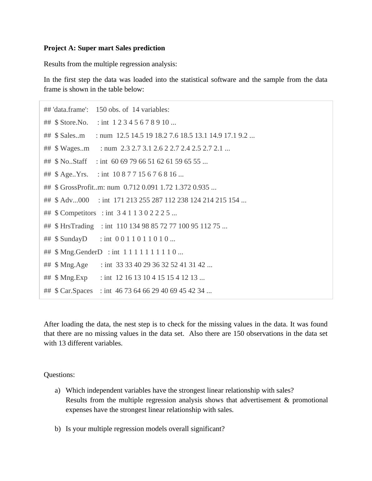
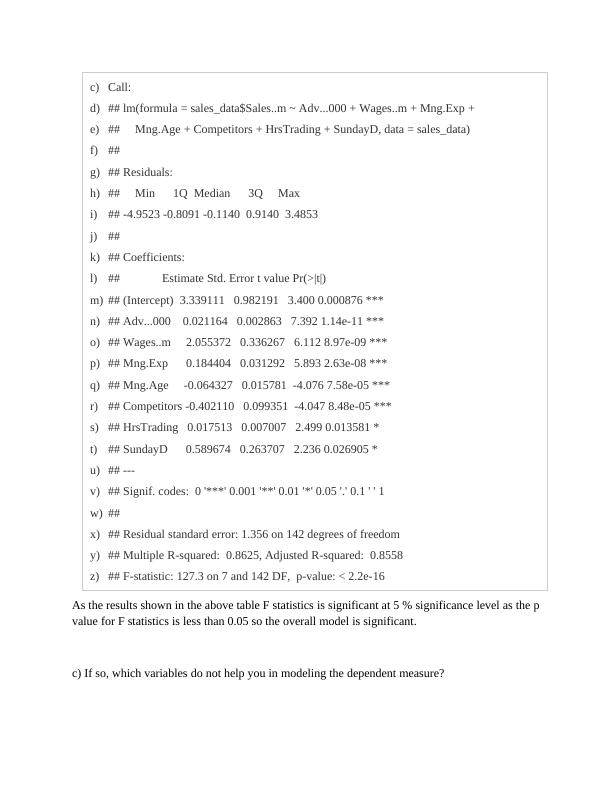
MIS171 - Business Analytics Assignment
Deakin University
Business Analytics (MIS171)
Added on 2019-10-30
BookmarkShareRelated Documents
End of preview
Want to access all the pages? Upload your documents or become a member.
Development of a Multiple Regression Model for Sales Estimation
|12
|1908
|297
Analysis of Sales and Customers
|3
|779
|416
Data Analysis and Linear Programming
|7
|838
|160
Time Series Analysis for Ozone Layer Thickness
|19
|1811
|401
Management Analytics: Regression Analysis on Gender and Salary
|8
|1694
|411