Data Analysis Report: Transport Expenses, Calculations, Forecasting
VerifiedAdded on 2022/12/12
|9
|1349
|301
Homework Assignment
AI Summary
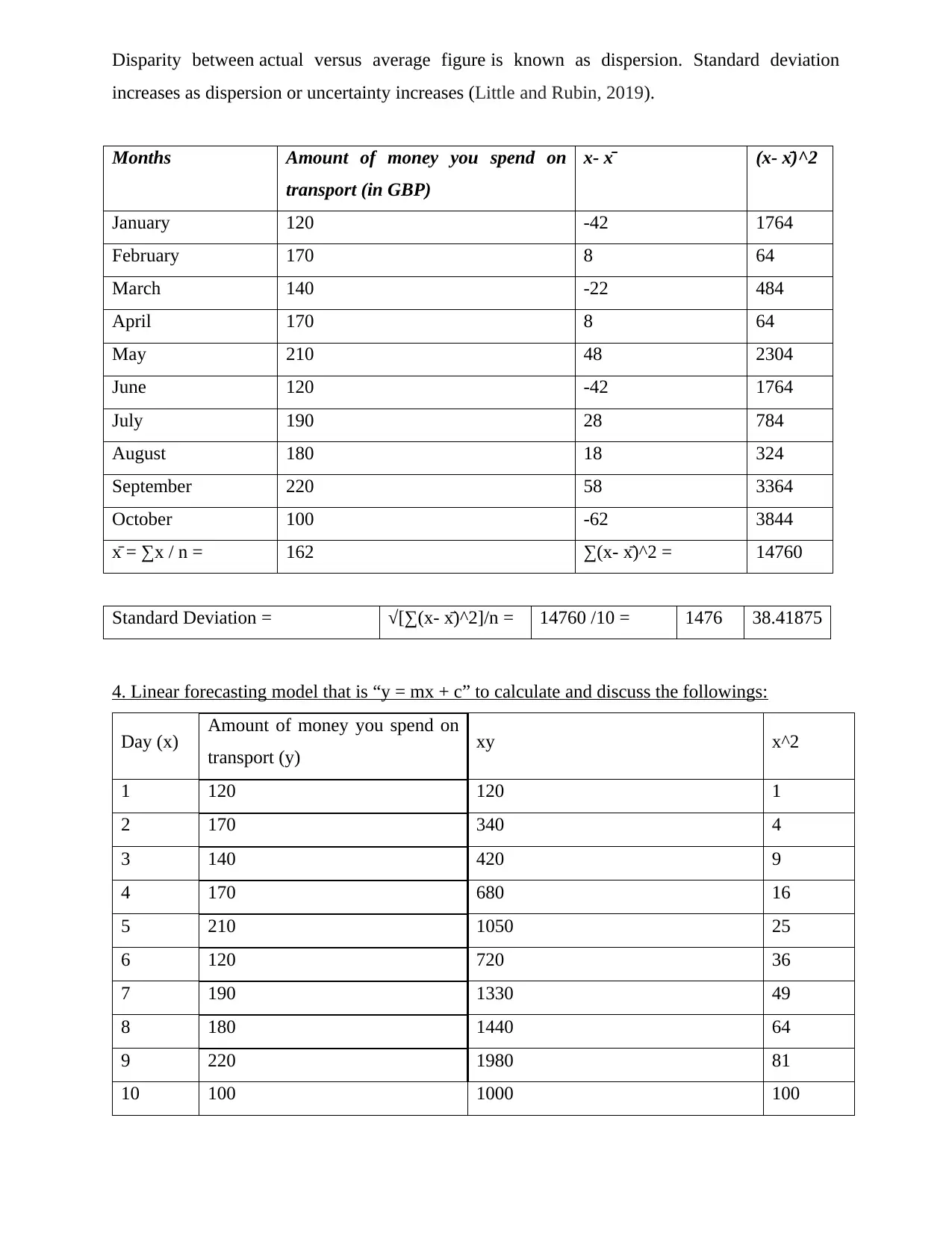
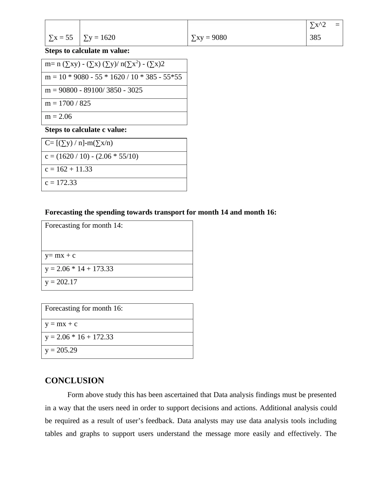
This assignment provides a comprehensive analysis of transport expenses over a ten-month period. It begins with arranging the expense data in a tabular format and then presents the data using both line and column charts for visual representation. The core of the assignment involves detailed calculations of statistical measures, including the mean, median, mode, range, and standard deviation. Furthermore, a linear forecasting model (y = mx + c) is applied to predict future spending on transport, specifically for months 14 and 16. The assignment concludes by summarizing the findings and highlighting the importance of data analysis in making informed decisions, supported by relevant references to statistical methods and data analysis techniques.


1 out of 9
Related Documents


Your All-in-One AI-Powered Toolkit for Academic Success.
+13062052269
info@desklib.com
Available 24*7 on WhatsApp / Email
![[object Object]](/_next/static/media/star-bottom.7253800d.svg)
Copyright © 2020–2026 A2Z Services. All Rights Reserved. Developed and managed by ZUCOL.