Propagation and Antennas
VerifiedAdded on 2023/03/31
|14
|2123
|154
AI Summary
This document discusses the expression for an N-element antenna array factor, the MATLAB code for plotting the array factor, the half-power beam width, and the three-array element alignment. It also provides the MATLAB code for plotting the array factor and calculates the energy stored in a cylindrical coordinate system.
Contribute Materials
Your contribution can guide someone’s learning journey. Share your
documents today.

Running head: PROPAGATION AND ANTENNAS 1
Propagation and Antennas
Name
Institution
Propagation and Antennas
Name
Institution
Secure Best Marks with AI Grader
Need help grading? Try our AI Grader for instant feedback on your assignments.
PROPAGATION AND ANTENNAS 2
Question 1
a0=1 , a1=2 , δ= π
2 , d= λ
4
The expression for an N-element antenna array factor is:
Fa ( θ ) =|∑
i=0
N−1
ai e j ψ 1
e jikdcos ( θ )
|
2
Since it is a two-element array, we substitute N=2 to get:
Fa ( θ ) =|∑
i=0
N−1
ai e j ψ 1
e jikdcos ( θ )
|
2
=|∑
i=0
2−1
ai e jψ1
e jikdcos ( θ )
|
2
=|∑
i=0
1
ai e j ψ1
e jikdcos ( θ )
|
2
¿|a0 e j ψ0
e j (0 )kdcos (θ ) +a1 e j ψ 1
e j(1)kdcos (θ )
|2
¿|a0 +a1 e j δ e j ( 2 π
λ ) dcos ( θ )
|
2
Substituting the values for a0 , a1 , δ ,∧dwe get:
Fa ( θ )=|1+2 e j ( π
2 ) e j ( 2 π
λ )( λ
4 )cos (θ )
|2
=|1+2 e j ( π
2 ) e j ( π
2 )cos (θ )
|2
¿|1+2 e j ( π
2 ) cos ( θ ) + j ( π
2 )|
2
=|1+2 e j ( π
2 ) ( cos ( θ ) +1 )
|
2
¿
|1+2 [ cos ( π
2 ( cos ( θ ) +1 ) ) + jsin ( π
2 ( cos ( θ ) +1 ) ) ]|
2
¿
|1+2 cos ( π
2 ( cos ( θ ) +1 ) )|2
+
|2 sin ( π
2 ( cos ( θ )+ 1 ))|2
¿ 1+4 cos ( π
2 ( cos ( θ ) +1 ) )+ 4 co s2
( π
2 ( cos ( θ ) +1 ) )+4 si n2
( π
2 ( cos ( θ )+1 ) )
¿ 1+4 cos ( π
2 ( cos ( θ ) +1 ) )+ 4 {co s2
( π
2 ( cos (θ ) +1 ) )+ si n2
( π
2 ( cos ( θ )+1 ) ) }
¿ 1+4 cos ( π
2 ( cos ( θ ) +1 ) )+ 4 (1)
PROPAGATION AND ANTENNAS 3
¿ 5+ 4 cos ( π
2 ( cos ( θ ) +1 ) )
Therefore, the array factor Fa ( θ ) =5+4 cos ( π
2 ( cos ( θ ) +1 ) )
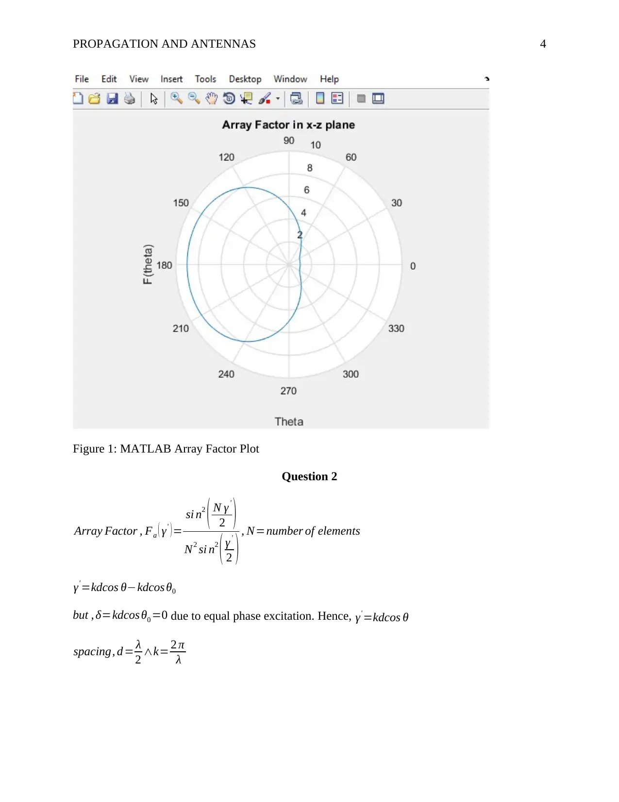
The plot of the array factor in MATLAB using the code below is shown I figure 1.
%MATLAB code for plotting array factor
clear all;
% Defining theta range
F = zeros(1,360);
for theta=1:360
% change degree to radian
deg2rad(theta) = (theta*pi)/180;
%array factor calculation
F(theta) =abs(5+4*cos(pi/2*(cos(deg2rad(theta))+1)));
end
% plot the array factor
polar(deg2rad,F);
%Title and Axis Labels
title('Array Factor in x-z plane');
xlabel('Theta');
ylabel('F(theta)');
¿ 5+ 4 cos ( π
2 ( cos ( θ ) +1 ) )
Therefore, the array factor Fa ( θ ) =5+4 cos ( π
2 ( cos ( θ ) +1 ) )
The plot of the array factor in MATLAB using the code below is shown I figure 1.
%MATLAB code for plotting array factor
clear all;
% Defining theta range
F = zeros(1,360);
for theta=1:360
% change degree to radian
deg2rad(theta) = (theta*pi)/180;
%array factor calculation
F(theta) =abs(5+4*cos(pi/2*(cos(deg2rad(theta))+1)));
end
% plot the array factor
polar(deg2rad,F);
%Title and Axis Labels
title('Array Factor in x-z plane');
xlabel('Theta');
ylabel('F(theta)');
PROPAGATION AND ANTENNAS 4
Figure 1: MATLAB Array Factor Plot
Question 2
Array Factor , Fa ( γ' ) =
si n2
( N γ '
2 )
N2 si n2
( γ '
2 ) , N=number of elements
γ'=kdcos θ−kdcos θ0
but , δ=kdcos θ0 =0 due to equal phase excitation. Hence, γ' =kdcos θ
spacing, d = λ
2 ∧k= 2 π
λ
Figure 1: MATLAB Array Factor Plot
Question 2
Array Factor , Fa ( γ' ) =
si n2
( N γ '
2 )
N2 si n2
( γ '
2 ) , N=number of elements
γ'=kdcos θ−kdcos θ0
but , δ=kdcos θ0 =0 due to equal phase excitation. Hence, γ' =kdcos θ
spacing, d = λ
2 ∧k= 2 π
λ
Secure Best Marks with AI Grader
Need help grading? Try our AI Grader for instant feedback on your assignments.
PROPAGATION AND ANTENNAS 5
Fa ( θ )=
si n2
( 6 × 2 π
λ × λ
2 cos θ
2 )
62 si n2
( 2 π
λ × λ
2 cos θ
2 ) = si n2 ( 3 π cos θ )
36 si n2
( π
2 cos θ )
Fa ( θ )= si n2 ( 3 π cos θ )
36 si n2
( π
2 cos θ )=
( sin (3 π cos θ )
6 sin ( π
2 cos θ ) )2
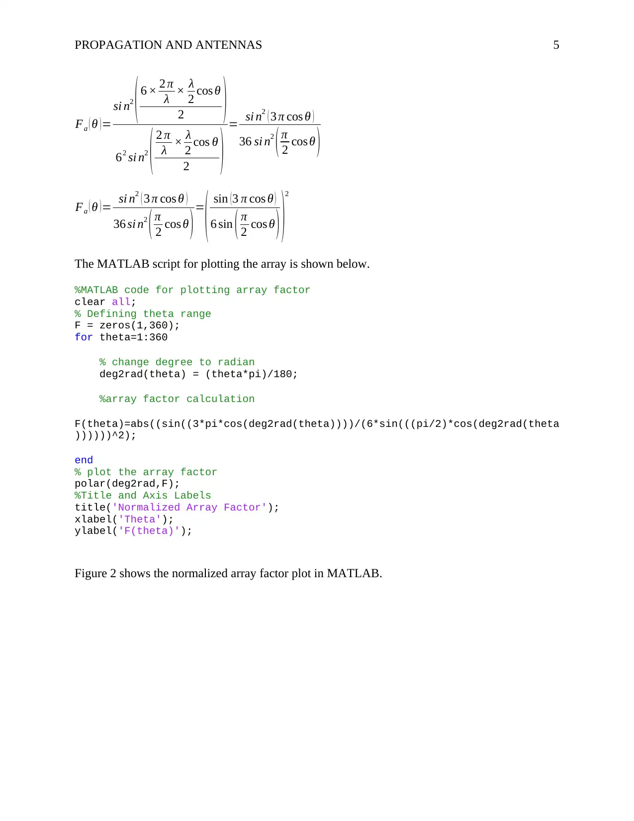
The MATLAB script for plotting the array is shown below.
%MATLAB code for plotting array factor
clear all;
% Defining theta range
F = zeros(1,360);
for theta=1:360
% change degree to radian
deg2rad(theta) = (theta*pi)/180;
%array factor calculation
F(theta)=abs((sin((3*pi*cos(deg2rad(theta))))/(6*sin(((pi/2)*cos(deg2rad(theta
))))))^2);
end
% plot the array factor
polar(deg2rad,F);
%Title and Axis Labels
title('Normalized Array Factor');
xlabel('Theta');
ylabel('F(theta)');
Figure 2 shows the normalized array factor plot in MATLAB.
Fa ( θ )=
si n2
( 6 × 2 π
λ × λ
2 cos θ
2 )
62 si n2
( 2 π
λ × λ
2 cos θ
2 ) = si n2 ( 3 π cos θ )
36 si n2
( π
2 cos θ )
Fa ( θ )= si n2 ( 3 π cos θ )
36 si n2
( π
2 cos θ )=
( sin (3 π cos θ )
6 sin ( π
2 cos θ ) )2
The MATLAB script for plotting the array is shown below.
%MATLAB code for plotting array factor
clear all;
% Defining theta range
F = zeros(1,360);
for theta=1:360
% change degree to radian
deg2rad(theta) = (theta*pi)/180;
%array factor calculation
F(theta)=abs((sin((3*pi*cos(deg2rad(theta))))/(6*sin(((pi/2)*cos(deg2rad(theta
))))))^2);
end
% plot the array factor
polar(deg2rad,F);
%Title and Axis Labels
title('Normalized Array Factor');
xlabel('Theta');
ylabel('F(theta)');
Figure 2 shows the normalized array factor plot in MATLAB.
PROPAGATION AND ANTENNAS 6
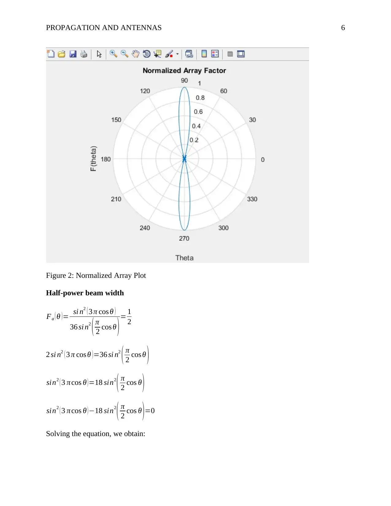
Figure 2: Normalized Array Plot
Half-power beam width
Fa ( θ )= si n2 ( 3 π cos θ )
36 si n2
( π
2 cos θ )= 1
2
2 si n2 ( 3 π cos θ )=36 si n2
( π
2 cos θ )
sin2 ( 3 π cos θ )=18 sin2
( π
2 cos θ )
sin2 ( 3 π cos θ )−18 sin2
( π
2 cos θ )=0
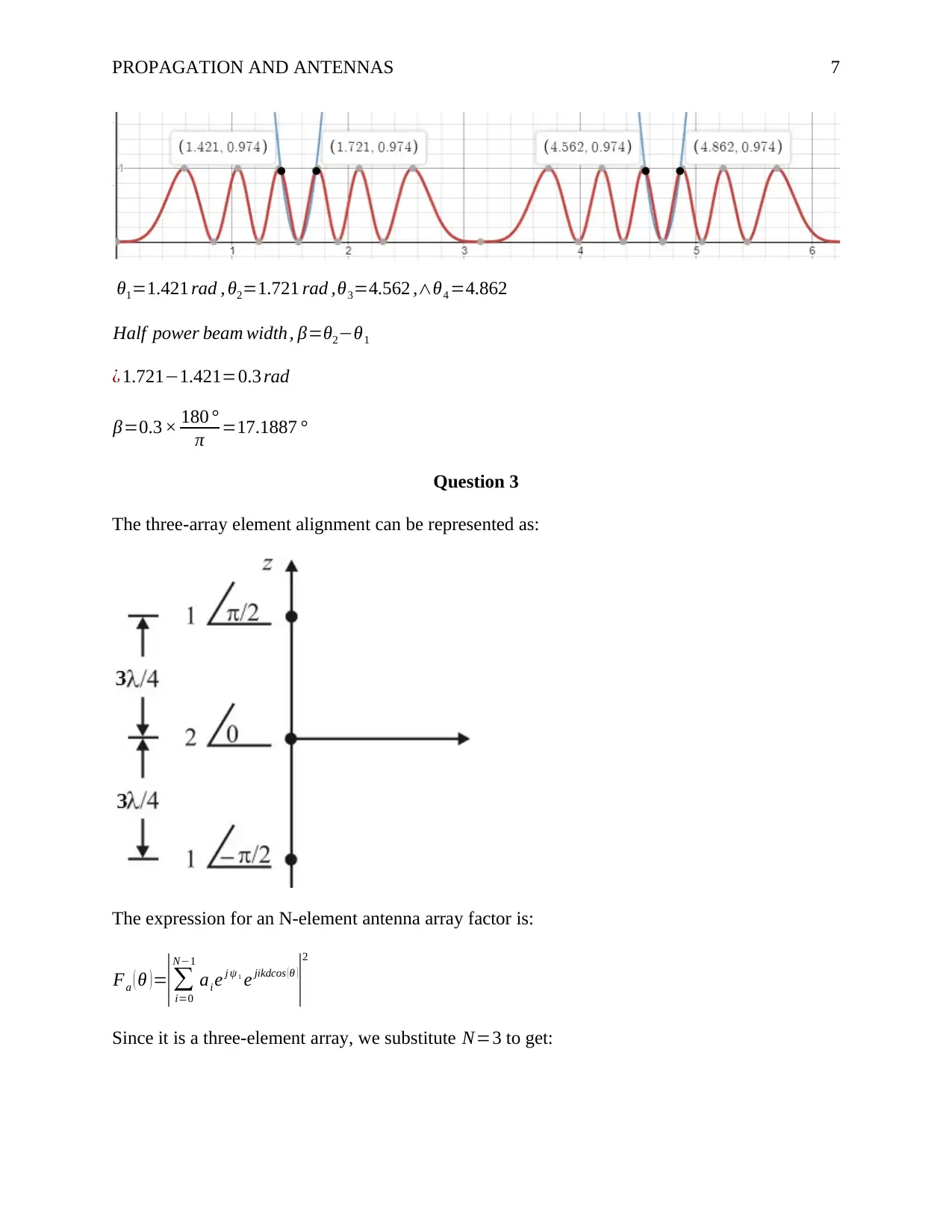
Solving the equation, we obtain:
Figure 2: Normalized Array Plot
Half-power beam width
Fa ( θ )= si n2 ( 3 π cos θ )
36 si n2
( π
2 cos θ )= 1
2
2 si n2 ( 3 π cos θ )=36 si n2
( π
2 cos θ )
sin2 ( 3 π cos θ )=18 sin2
( π
2 cos θ )
sin2 ( 3 π cos θ )−18 sin2
( π
2 cos θ )=0
Solving the equation, we obtain:
PROPAGATION AND ANTENNAS 7
θ1=1.421 rad , θ2=1.721 rad ,θ3=4.562 ,∧θ4 =4.862
Half power beam width, β=θ2−θ1
¿ 1.721−1.421=0.3 rad
β=0.3 × 180 °
π =17.1887 °
Question 3
The three-array element alignment can be represented as:
The expression for an N-element antenna array factor is:
Fa ( θ ) =|∑
i=0
N−1
ai e j ψ 1
e jikdcos ( θ )
|
2
Since it is a three-element array, we substitute N=3 to get:
Paraphrase This Document
Need a fresh take? Get an instant paraphrase of this document with our AI Paraphraser
PROPAGATION AND ANTENNAS 8
Fa ( θ ) =
|∑
i=0
N−1
ai e j ψ 1
e jikdcos ( θ )
|
2
=
|∑
i=0
3−1
ai e jψ 1
e jikdcos ( θ )
|
2
=
|∑
i=0
2
ai e j ψ1
e jikdcos ( θ )
|
2
¿|∑
i=0
2
ai e jψ i
e ji ( 2 π
λ )( 3 λ
4 )cos (θ )
|2
=|∑
i=0
2
ai e j ψi
e ji ( 3 π
2 )cos (θ )
|2
In such a scenario, a0=1 , a1=2 ,∧a2=1.
Also, ψ0=−π
2 , ψ1=0 ,∧ψ2= π
2
Fa ( θ )=|a0 e j ψ0
e j 0 3 π
2 cos ( θ )
+a1 e j ψ 1
e j 1 3 π
2 cos (θ )
+ a2 e jψ 2
e j 2 3 π
2 cos (θ )
|2
Fa ( θ )=|e
− jπ
2 +2 e
j 3 π
2 cos ( θ )
+e
jπ
2 e j 3 πcos (θ )
|2
Fa ( θ )=|− j+ 2cos ( 3 π
2 cos ( θ ) )+ j 2 sin ( 3 π
2 cos ( θ ) )+ jcos ( 3 πcos ( θ ) ) −sin ( 3 πcos (θ ) )|2
¿ ¿ ¿
¿|2 cos ( 3 π
2 cos ( θ ) ) −sin ( 3 πcos ( θ ) )|
2
+¿ ¿
¿ 4 co s2
( 3 π
2 cos ( θ ) )+si n2 ( 3 πcos ( θ ) )−4 cos ( 3 π
2 cos ( θ ) )sin ( 3 πcos ( θ ) )+ co s2 ( 3 πcos (θ ) ) +4 cos ( 3 πcos ( θ ) ) sin ( 3 π
2 c
Upon further simplification we get:
Fa ( θ ) =4 +1+4 [ −cos ( 3 π
2 cos ( θ ) ) sin ( 3 πcos ( θ ) ) + cos ( 3 πcos ( θ ) ) sin ( 3 π
2 cos ( θ ) ) ] +1−2 [ cos ( 3 πcos ( θ ) ) +2 sin ( 3 π
2 c
¿ 6−4 [ sin ( 3 πcos ( θ ) −3 π
2 cos ( θ ) ) ] −2 [ cos ( 3 πcos ( θ ) ) +2sin ( 3 π
2 cos ( θ ) ) ]
¿ 6−4 sin ( 3 π
2 cos ( θ ) )−2 cos ( 3 πcos ( θ ) ) −4 sin ( 3 π
2 cos ( θ ) )
Therefore , the array factor , Fa ( θ )=6−8 sin (3 π
2 cos ( θ ) )−2 cos ( 3 πcos ( θ ) )
The MATLAB code for plotting the array is shown below.
PROPAGATION AND ANTENNAS 9
%MATLAB code for plotting array factor
clear all;
% Defining theta range
F = zeros(1,360);
for theta=1:360
% change degree to radian
deg2rad(theta) = (theta*pi)/180;
%array factor calculation
F(theta)=6-8*sin(1.5*pi*cos(deg2rad(theta)))-
2*cos(3*pi*cos(deg2rad(theta)));
end
% plot the array factor
polar(deg2rad,F);
%Title and Axis Labels
title('Array Factor');
xlabel('Theta');
ylabel('F(theta)');
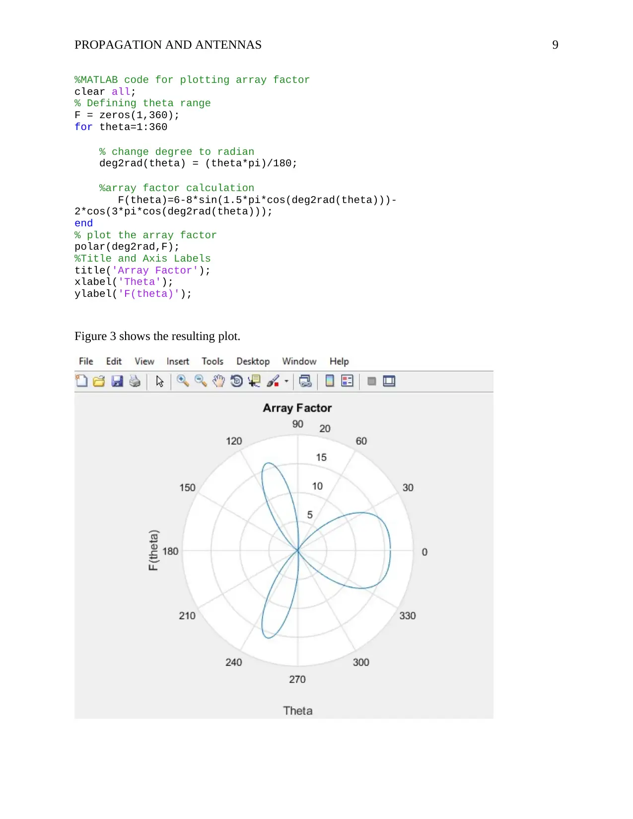
Figure 3 shows the resulting plot.
%MATLAB code for plotting array factor
clear all;
% Defining theta range
F = zeros(1,360);
for theta=1:360
% change degree to radian
deg2rad(theta) = (theta*pi)/180;
%array factor calculation
F(theta)=6-8*sin(1.5*pi*cos(deg2rad(theta)))-
2*cos(3*pi*cos(deg2rad(theta)));
end
% plot the array factor
polar(deg2rad,F);
%Title and Axis Labels
title('Array Factor');
xlabel('Theta');
ylabel('F(theta)');
Figure 3 shows the resulting plot.
PROPAGATION AND ANTENNAS 10
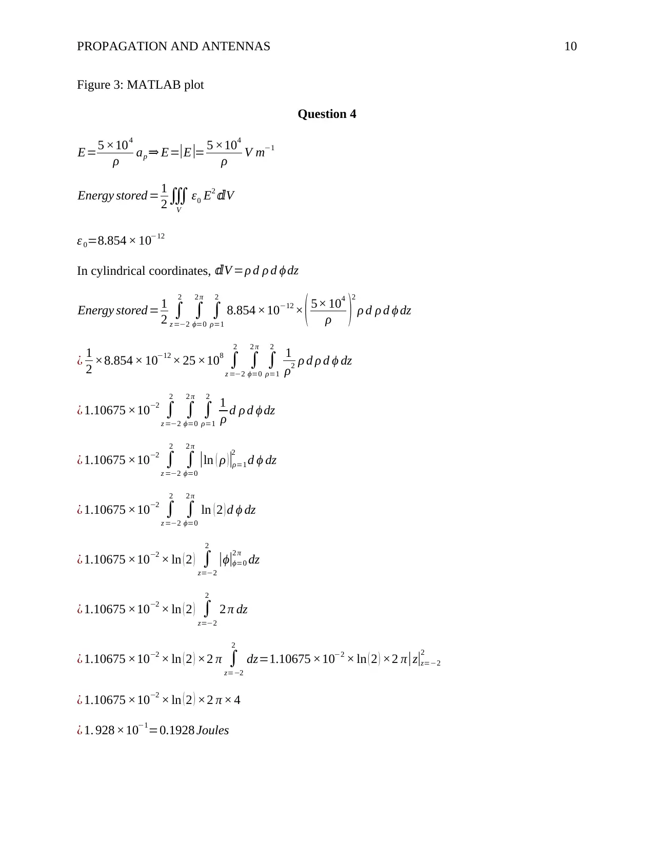
Figure 3: MATLAB plot
Question 4
E=5 ×10⁴
ρ ap ⇒ E=|E |= 5 ×10⁴
ρ V m−1
Energy stored = 1
2∭
V
ε0 E2 Vⅆ
ε 0=8.854 × 10⁻¹²
In cylindrical coordinates, Vⅆ =ρ d ρ d ϕ dz
Energy stored = 1
2 ∫
z =−2
2
∫
ϕ=0
2 π
∫
ρ=1
2
8.854 ×10⁻¹² × ( 5× 10⁴
ρ )2
ρ d ρ d ϕ dz
¿ 1
2 ×8.854 × 10−12 × 25 ×108
∫
z =−2
2
∫
ϕ=0
2 π
∫
ρ=1
2
1
ρ2 ρ d ρ d ϕ dz
¿ 1.10675 ×10⁻²
∫
z =−2
2
∫
ϕ=0
2 π
∫
ρ=1
2
1
ρ d ρ d ϕ dz
¿ 1.10675 ×10⁻²
∫
z =−2
2
∫
ϕ=0
2 π
|ln ( ρ )|ρ=1
2
d ϕ dz
¿ 1.10675 ×10⁻²
∫
z =−2
2
∫
ϕ=0
2 π
ln ( 2 ) d ϕ dz
¿ 1.10675 ×10⁻² × ln ( 2 ) ∫
z=−2
2
|ϕ|ϕ=0
2 π
dz
¿ 1.10675 ×10⁻² × ln ( 2 ) ∫
z=−2
2
2 π dz
¿ 1.10675 ×10⁻² × ln ( 2 ) ×2 π ∫
z=−2
2
dz=1.10675 ×10⁻² × ln ( 2 ) ×2 π |z|z=−2
2
¿ 1.10675 ×10⁻² × ln ( 2 ) ×2 π × 4
¿ 1. 928 ×10−1=0.1928 Joules
Secure Best Marks with AI Grader
Need help grading? Try our AI Grader for instant feedback on your assignments.
PROPAGATION AND ANTENNAS 11
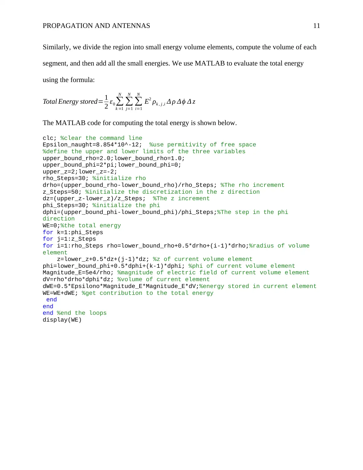
Similarly, we divide the region into small energy volume elements, compute the volume of each
segment, and then add all the small energies. We use MATLAB to evaluate the total energy
using the formula:
Total Energy stored= 1
2 ε0 ∑
k =1
N
∑
j=1
N
∑
i=1
N
E2 ρk , j ,i Δ ρ Δϕ Δ z
The MATLAB code for computing the total energy is shown below.
clc; %clear the command line
Epsilon_naught=8.854*10^-12; %use permitivity of free space
%define the upper and lower limits of the three variables
upper_bound_rho=2.0;lower_bound_rho=1.0;
upper_bound_phi=2*pi;lower_bound_phi=0;
upper_z=2;lower_z=-2;
rho_Steps=30; %initialize rho
drho=(upper_bound_rho-lower_bound_rho)/rho_Steps; %The rho increment
z_Steps=50; %initialize the discretization in the z direction
dz=(upper_z-lower_z)/z_Steps; %The z increment
phi_Steps=30; %initialize the phi
dphi=(upper_bound_phi-lower_bound_phi)/phi_Steps;%The step in the phi
direction
WE=0;%the total energy
for k=1:phi_Steps
for j=1:z_Steps
for i=1:rho_Steps rho=lower_bound_rho+0.5*drho+(i-1)*drho;%radius of volume
element
z=lower_z+0.5*dz+(j-1)*dz; %z of current volume element
phi=lower_bound_phi+0.5*dphi+(k-1)*dphi; %phi of current volume element
Magnitude_E=5e4/rho; %magnitude of electric field of current volume element
dV=rho*drho*dphi*dz; %volume of current element
dWE=0.5*Epsilono*Magnitude_E*Magnitude_E*dV;%energy stored in current element
WE=WE+dWE; %get contribution to the total energy
end
end
end %end the loops
display(WE)
PROPAGATION AND ANTENNAS 12
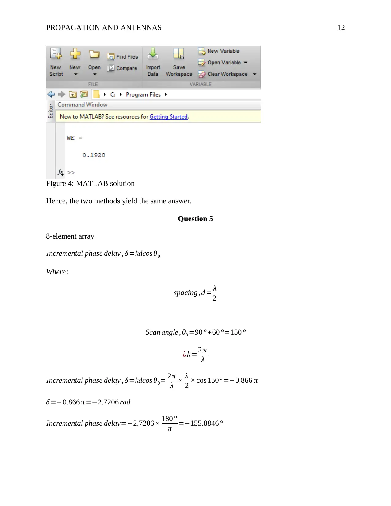
Figure 4: MATLAB solution
Hence, the two methods yield the same answer.
Question 5
8-element array
Incremental phase delay , δ=kdcos θ0
Where :
spacing, d = λ
2
Scan angle, θ0 =90 °+60 °=150 °
¿ k =2 π
λ
Incremental phase delay , δ=kdcos θ0= 2 π
λ × λ
2 × cos 150° =−0.866 π
δ=−0.866 π =−2.7206 rad
Incremental phase delay=−2.7206× 180 °
π =−155.8846 °
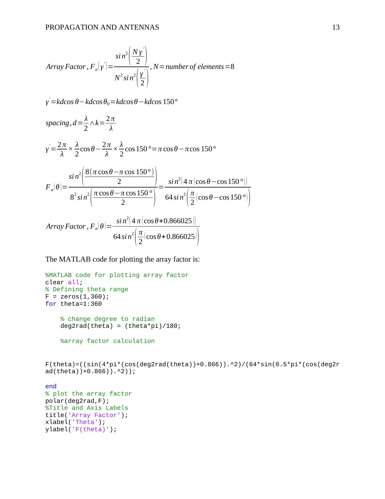
PROPAGATION AND ANTENNAS 13
Array Factor , Fa ( γ' ) =
si n2
( N γ '
2 )
N2 si n2
( γ '
2 ) , N=number of elements=8
γ' =kdcos θ−kdcos θ0 =kdcos θ−kdcos 150°
spacing, d = λ
2 ∧k= 2 π
λ
γ'= 2 π
λ × λ
2 cos θ− 2 π
λ × λ
2 cos 150 °=π cos θ−π cos 150°
Fa ( θ )=
si n2
( 8(π cos θ−π cos 150°)
2 )
82 si n2
( π cos θ−π cos 150 °
2 ) = si n2 ( 4 π ( cos θ−cos 150 ° ) )
64 si n2
( π
2 ( cos θ−cos 150 ° ) )
Array Factor , Fa ( θ )= si n2 ( 4 π ( cos θ+0.866025 ) )
64 si n2
( π
2 ( cos θ+ 0.866025 ) )
The MATLAB code for plotting the array factor is:
%MATLAB code for plotting array factor
clear all;
% Defining theta range
F = zeros(1,360);
for theta=1:360
% change degree to radian
deg2rad(theta) = (theta*pi)/180;
%array factor calculation
F(theta)=((sin(4*pi*(cos(deg2rad(theta))+0.866)).^2)/(64*sin(0.5*pi*(cos(deg2r
ad(theta))+0.866)).^2));
end
% plot the array factor
polar(deg2rad,F);
%Title and Axis Labels
title('Array Factor');
xlabel('Theta');
ylabel('F(theta)');
Paraphrase This Document
Need a fresh take? Get an instant paraphrase of this document with our AI Paraphraser
PROPAGATION AND ANTENNAS 14
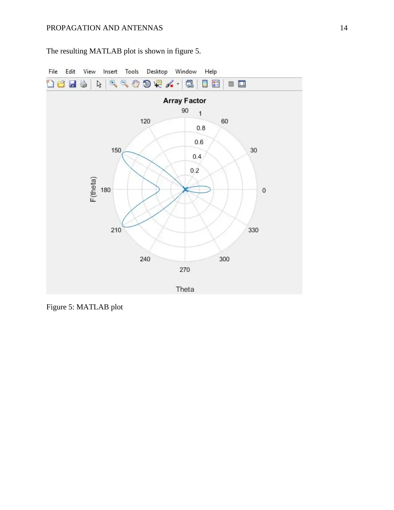
The resulting MATLAB plot is shown in figure 5.
Figure 5: MATLAB plot
The resulting MATLAB plot is shown in figure 5.
Figure 5: MATLAB plot
1 out of 14
Related Documents


Your All-in-One AI-Powered Toolkit for Academic Success.
+13062052269
info@desklib.com
Available 24*7 on WhatsApp / Email
![[object Object]](/_next/static/media/star-bottom.7253800d.svg)
Unlock your academic potential
© 2024 | Zucol Services PVT LTD | All rights reserved.