Energy Resources & Utilization Lab Reports - UET Lahore 2018-ME-133
VerifiedAdded on 2024/01/18
|71
|15066
|477
AI Summary
This document contains a compilation of Energy Resources and Utilization (ERU) lab reports from the University of Engineering and Technology (UET) Lahore, specifically for the course code 2018-ME-133. The reports cover a range of experiments including the study of a pyrheliometer for calculating Direct Normal Irradiance (DNI) and Global Horizontal Irradiance (GHI), experiments related to solar radiation and evacuated tube collectors, analysis of parabolic trough collectors, wind tunnel experiments, and the study of dynamometers. Each lab report includes objectives, literature review, experimental setup, procedures, results, conclusions, advantages, disadvantages (where applicable), and references, providing a comprehensive understanding of each topic. The reports also incorporate graphs, figures, and schematic diagrams to aid in the visualization and analysis of the experimental data.
ERU-Lab Reports 2018-ME-133
University of Engineering and Technology
Lahore
Assignment of:
Energy Resources and Utilization-Laboratory
Assignment Type:
Lab Report
Submitted To:
Sir Syed Saqib
Submitted By:
2018-ME-133
Ahsan Junaid
________________________________________________________________
University of Engineering and Technology
Lahore
Assignment of:
Energy Resources and Utilization-Laboratory
Assignment Type:
Lab Report
Submitted To:
Sir Syed Saqib
Submitted By:
2018-ME-133
Ahsan Junaid
________________________________________________________________
Paraphrase This Document
Need a fresh take? Get an instant paraphrase of this document with our AI Paraphraser
ERU-Lab Reports 2018-ME-133
Table of Contents
1. Objective: ............................................................................................................. 8
2. Experimental Setup: ............................................................................................. 8
3. Literature Review ................................................................................................ 9
3.1. Pyrheliometer: ................................................................................................. 9
3.2. Main Components of Pyrheliometer: ............................................................. 9
3.3. Pyrheliometer a Solar Irriadiance Sensor: ....................................................10
3.4. Difference between Pyrheliometer & Pyranometer: ....................................10
3.5. Direct Normal Irradiance (DNI): ..................................................................11
3.6. Global Horizontal Irradiance (GHI): ............................................................11
4. Working of a Pyrheliometer: .............................................................................11
5. Procedure: ..........................................................................................................12
6. Advantages of Pyrheliometer: ...........................................................................13
7. Applications of Pyrheliometer: ..........................................................................13
8. Characteristics of Pyrheliometer: ......................................................................16
9. References ..........................................................................................................16
1. Objective ............................................................................................................17
2. Literature Review ..............................................................................................17
2.1. Declination: ...................................................................................................18
2.2. Solar elevation ..............................................................................................19
Zenith angle ..........................................................................................................19
Solar Azimuth Angle: ...........................................................................................19
3. Procedure: ..........................................................................................................20
4. Graphs ................................................................................................................21
5. Conclusion .........................................................................................................21
6. Advantages: .......................................................................................................22
7. Disadvantages: ...................................................................................................22
ERU-Lab Reports 2018-ME-133
8. References:.........................................................................................................23
1. Objective: ...........................................................................................................24
2. Experimental Setup ............................................................................................24
3. Literature Review ..............................................................................................25
3.1. Evacuated Tube Collectors ...........................................................................25
3.1.3.1 Direct-flow evacuated-tube collectors: ...................................................27
3.1.3.2 Heat pipe evacuated-tube collectors: ....................................................28
Integrated Tank Solar Collectors: .........................................................................29
4. Experimental Setup: ...........................................................................................30
5. Measuring Instruments and device: ...................................................................30
6. Experimentation Data Analysis: ........................................................................30
6.1. Experimental Results: ...................................................................................31
7. Conclusion: ........................................................................................................31
8. References ..........................................................................................................32
1. Objective ............................................................................................................33
2. Literature Review ..............................................................................................33
2.1. Parabolic Trough Collector: ........................................................................33
2.1.1. Working Principle ....................................................................................34
2.1.2. Solar Thermal Power System ...................................................................34
2.1.2.2. Solar Power Towers ..............................................................................35
2.1.2.3. Solar Dish Systems ...............................................................................35
3. Optical and Thermal Analysis of High Concentration Parabolic Trough
Collectors .................................................................................................................37
3.1. Structure ......................................................................................................37
3.1.1. Geometry: ..................................................................................................37
3.1.2. Solar Tracking: ..........................................................................................37
3.1.3. Reflectors: ...................................................................................................37
3.1.3.1. Photogrammetry: ....................................................................................37
3.1.3.2. Deflectometry: ........................................................................................38
⊘ This is a preview!⊘
Do you want full access?
Subscribe today to unlock all pages.
Trusted by 1+ million students worldwide
ERU-Lab Reports 2018-ME-133
3.1.4. Reflectivity Measurement: .........................................................................39
4. Abrasion Test: ....................................................................................................39
5. Advantages: .......................................................................................................40
6. Disadvantages: ...................................................................................................40
7. References ..........................................................................................................41
1. Objective: ...........................................................................................................42
2. Experimental Setup: ...........................................................................................42
3. Theory: ...............................................................................................................43
4. Procedure: ..........................................................................................................44
5. Calculations and observations: ..........................................................................45
6. Result .................................................................................................................47
7. References ..........................................................................................................48
1. Objective: ...........................................................................................................49
2. Literature Review ..............................................................................................49
2.1. Dynamometer: ...............................................................................................49
2.2. Ac dynamometer: ..........................................................................................50
2.3. Types of Dynamometers: ..............................................................................51
2.3.1. Eddy Current Dynamometer ....................................................................51
2.4. Applications for Dynamometers .................................................................53
2.4.1. Data Acquisition .......................................................................................54
2.5. Dynamometer Design for measuring the cutting force on Turning ............54
2.6. Data acquisition ...........................................................................................55
2.7. Advantages ..................................................................................................56
2.8. Disadvantages: .............................................................................................56
3. Rpm and rotating torque ....................................................................................56
4. Results: ...............................................................................................................57
5. References:.........................................................................................................58
1. Objective ............................................................................................................59
2. Experimental Setup ............................................................................................59
Paraphrase This Document
Need a fresh take? Get an instant paraphrase of this document with our AI Paraphraser
ERU-Lab Reports 2018-ME-133
3. Literature View ..................................................................................................59
3.1. Wind Tunnel ..................................................................................................59
3.2. “Types of wind tunnels” ...............................................................................60
3.2.1. “Open vs closed circuit wind tunnel” .......................................................60
3.2.2. “Subsonic vs Supersonic wind tunnel” ...................................................61
3.2.3. “Education vs research wind tunnel” .......................................................62
3.2.4. “Laminar vs turbulent wind tunnel” ........................................................62
3.3. Parts of Wind Tunnel ....................................................................................62
a. “Inlet duct” .....................................................................................................62
b. “Test section” ..............................................................................................62
c. “Diffuser” .......................................................................................................63
d. “Axial flow fan unit” ...................................................................................63
e. “Control console” ...........................................................................................63
f. “Attachments” ................................................................................................63
i. “Strain gauge balance” ...................................................................................63
ii. “Multi bank manometer” .............................................................................63
3.4. Aerodynamics Fundamentals ......................................................................64
Expression For “Lift Force” .................................................................................65
4. Procedure ...........................................................................................................67
5. Results ................................................................................................................67
6. Graphs ................................................................................................................68
7. Simulation using Ansys .....................................................................................69
8. Conclusion and Recommendations ...................................................................70
9. References ..........................................................................................................71
ERU-Lab Reports 2018-ME-133
Table of Figures.
Figure 1 Measurement of Direct Normal Irridiance (DNI) using Pyrheliometer ...... 8
Figure 2 Measurement of Global Horizontal Irridiance (GHI) using Pryheliometer
.................................................................................................................................... 8
Figure 3 A Pyrheliometer pointed at the Sun to measure the Solar Irridiance
coming directly from the Sun .................................................................................... 9
Figure 4 Main Components of a Pyrheliometer........................................................ 9
Figure 5 Pyrometers measure Direct Solar radiation ..............................................10
Figure 6 Spectral Distribution of DNI – Data from ASTM G-173-03 Referance
Spectra. Red line shows typical spectral response curve of Quartz ........................11
Figure 7 DNI as measured by DR30 Pyrheliometer ...............................................12
Figure 8 Pyrheliometers measure only sunlight from a small area around the sun,
characterized by an opening half-angle of 2.5 ° ......................................................12
Figure 9 Standard Pyrheliometer Angles ................................................................13
Figure 10 Pyrheliometer in Scientific Metrological ...............................................14
Figure 11 Observations of Climate .........................................................................14
Figure 12 Testing Research of Material .................................................................14
Figure 13 Estimation of Solar Collector Efficiency ...............................................15
Figure 14 Use in PV Devices ..................................................................................15
Figure 15 Production of electricity from solar energy on large scale .....................17
Figure 16 Solar Zenith angle ....................................................................................19
Figure 17 Solar Azimuth Angle ...............................................................................19
Figure 18 Variance of reflectance with angle of incidence .....................................21
Figure 19 Experimental Setup .................................................................................24
Figure 20 Schematic Diagram of Evacuated Tube Collector ..................................25
Figure 21 A typical example of Digital Display ......................................................27
Figure 22 A Typical Diagram of components of Evacuated Tube Collector ..........27
Figure 23 Schematic Diagram of Direct flow Evacuated Tube Solar Collector .....28
Figure 24 Integrated Tank Solar Collectors ............................................................29
Figure 25 Parabolic Trough Collector ....................................................................33
Figure 26 Parabolic Trough Collector with single axis solar tracker .....................34
Figure 27 Linear Fresnel Reflectors ........................................................................35
Figure 28 Solar Power Towers ................................................................................35
Figure 29 Solar Dish systems ..................................................................................35
⊘ This is a preview!⊘
Do you want full access?
Subscribe today to unlock all pages.
Trusted by 1+ million students worldwide
ERU-Lab Reports 2018-ME-133
Figure 30 Analysis by photogrammetry of a common collector element ...............38
Figure 31 Measurement principle of Deflectometry of a reflecting surface ...........38
Figure 32 The bar projection field for the deflectometry and the reflecting image
on the mirrors of an inspected heliostat ...................................................................39
Figure 33 Sketch of the laser scanner VSHOT ........................................................39
Figure 34 Graph for Diurnal wind speed variations ...............................................45
Figure 35 Daily maximum, minimum, and mean wind speed variations ................46
Figure 36 Monthly mean speed wind variation .....................................................46
Figure 37 Schematic Diagram of Dynamometer .....................................................50
Figure 38 Eddy Current Dynamometer ...................................................................51
Figure 39 Power Dynamometer ...............................................................................52
Figure 40 Engine Dynamometer ..............................................................................53
Figure 41 Schematic representation of experimental set-up. .................................55
Figure 42 The photo of designed and developed dynamometer. .............................55
Figure 43 Graph between Damage and Torque .......................................................56
Figure 44 Transmission Dynamometer ....................................................................57
Figure 45 A typical Wind tunnel .............................................................................59
Figure 46 A schematic of wind tunnel .....................................................................60
Figure 47 Diagram of an open-circuit wind Tunnel ................................................60
Figure 48 Closed Circuit Wind Tunnel ....................................................................61
Figure 49 Wind Tunnel Design by NASA ...............................................................61
Figure 50 Schematic diagram of forces acting on a wind blade ..............................64
Figure 51Pressure and viscous forces acting on a differential element of an area of
wind blade ................................................................................................................64
Figure 52 Lift Force acting on a small particle. .......................................................65
Figure 53 Patterns of flow around air foil ...............................................................66
Figure 54 A graph between Lift force and Velocity ................................................68
Figure 55 A graph between Drag force and Velocity ..............................................68
Figure 56 Tip vortex at nominal wind speed 12 m/s ...............................................69
University of Engineering & Technology, Lahore
Paraphrase This Document
Need a fresh take? Get an instant paraphrase of this document with our AI Paraphraser
ERU-Lab Reports 2018-ME-133
Experiment No. 1
“Study of Pyrheliometer to Calculate Direct Normal
Irradiance and Global Horizontal Irradiance”
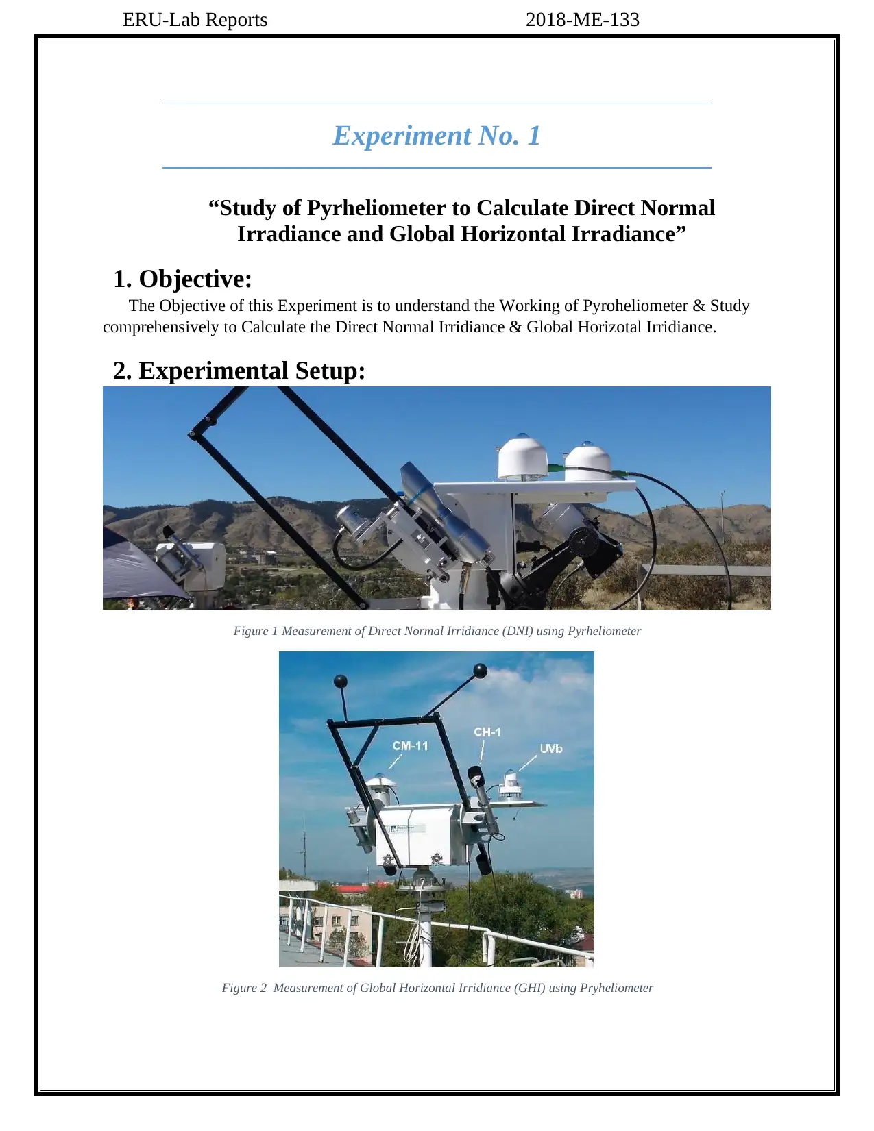
1. Objective:
The Objective of this Experiment is to understand the Working of Pyroheliometer & Study
comprehensively to Calculate the Direct Normal Irridiance & Global Horizotal Irridiance.
2. Experimental Setup:
Figure 1 Measurement of Direct Normal Irridiance (DNI) using Pyrheliometer
Figure 2 Measurement of Global Horizontal Irridiance (GHI) using Pryheliometer
Experiment No. 1
“Study of Pyrheliometer to Calculate Direct Normal
Irradiance and Global Horizontal Irradiance”
1. Objective:
The Objective of this Experiment is to understand the Working of Pyroheliometer & Study
comprehensively to Calculate the Direct Normal Irridiance & Global Horizotal Irridiance.
2. Experimental Setup:
Figure 1 Measurement of Direct Normal Irridiance (DNI) using Pyrheliometer
Figure 2 Measurement of Global Horizontal Irridiance (GHI) using Pryheliometer
ERU-Lab Reports 2018-ME-133
3. Literature Review
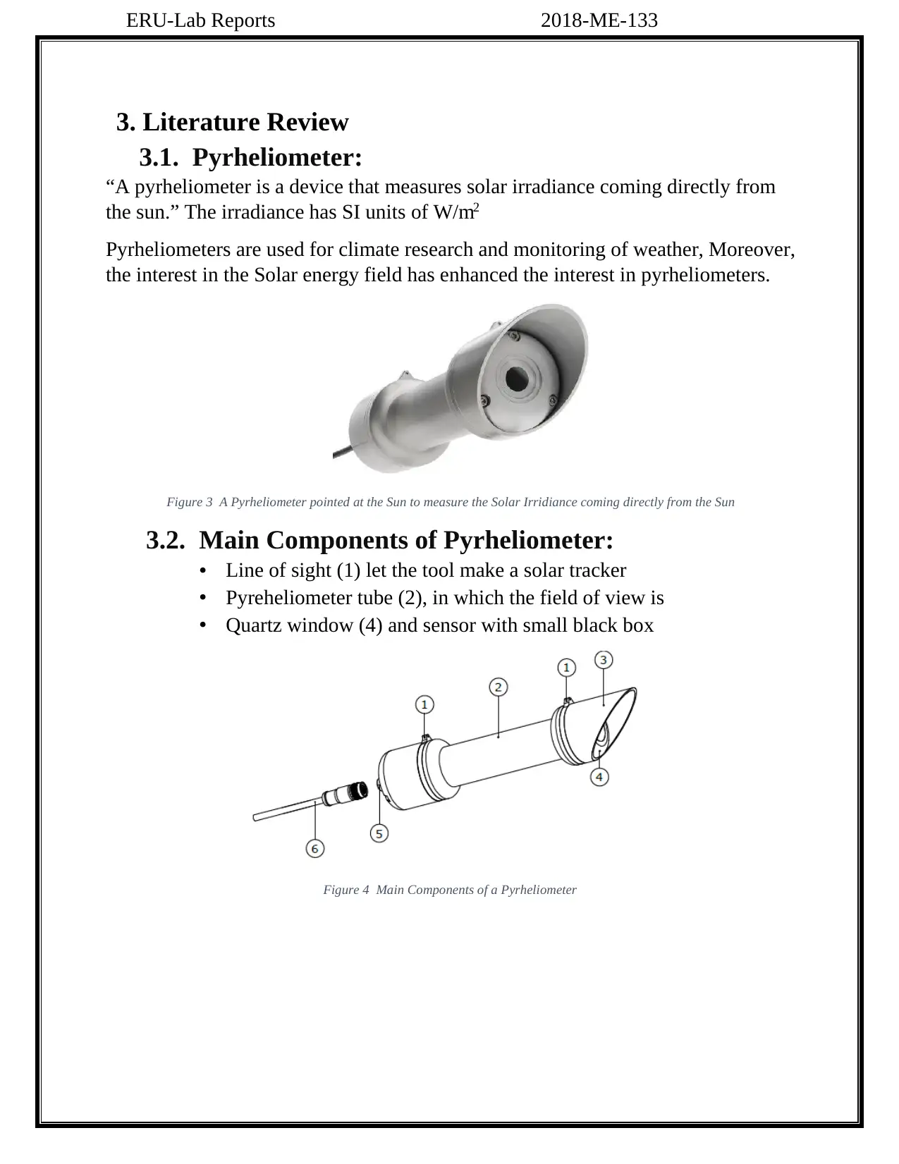
3.1. Pyrheliometer:
“A pyrheliometer is a device that measures solar irradiance coming directly from
the sun.” The irradiance has SI units of W/m2
Pyrheliometers are used for climate research and monitoring of weather, Moreover,
the interest in the Solar energy field has enhanced the interest in pyrheliometers.
Figure 3 A Pyrheliometer pointed at the Sun to measure the Solar Irridiance coming directly from the Sun
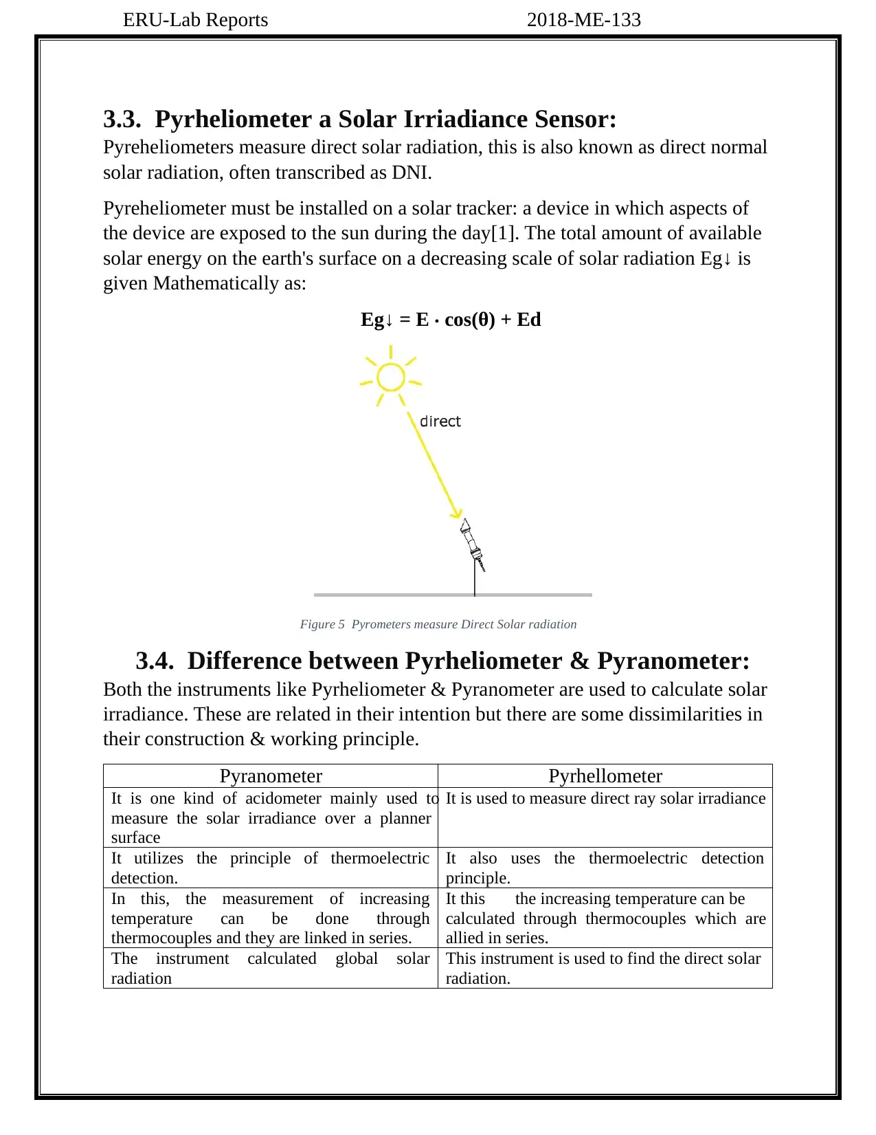
3.2. Main Components of Pyrheliometer:
• Line of sight (1) let the tool make a solar tracker
• Pyreheliometer tube (2), in which the field of view is
• Quartz window (4) and sensor with small black box
Figure 4 Main Components of a Pyrheliometer
3. Literature Review
3.1. Pyrheliometer:
“A pyrheliometer is a device that measures solar irradiance coming directly from
the sun.” The irradiance has SI units of W/m2
Pyrheliometers are used for climate research and monitoring of weather, Moreover,
the interest in the Solar energy field has enhanced the interest in pyrheliometers.
Figure 3 A Pyrheliometer pointed at the Sun to measure the Solar Irridiance coming directly from the Sun
3.2. Main Components of Pyrheliometer:
• Line of sight (1) let the tool make a solar tracker
• Pyreheliometer tube (2), in which the field of view is
• Quartz window (4) and sensor with small black box
Figure 4 Main Components of a Pyrheliometer
⊘ This is a preview!⊘
Do you want full access?
Subscribe today to unlock all pages.
Trusted by 1+ million students worldwide
ERU-Lab Reports 2018-ME-133
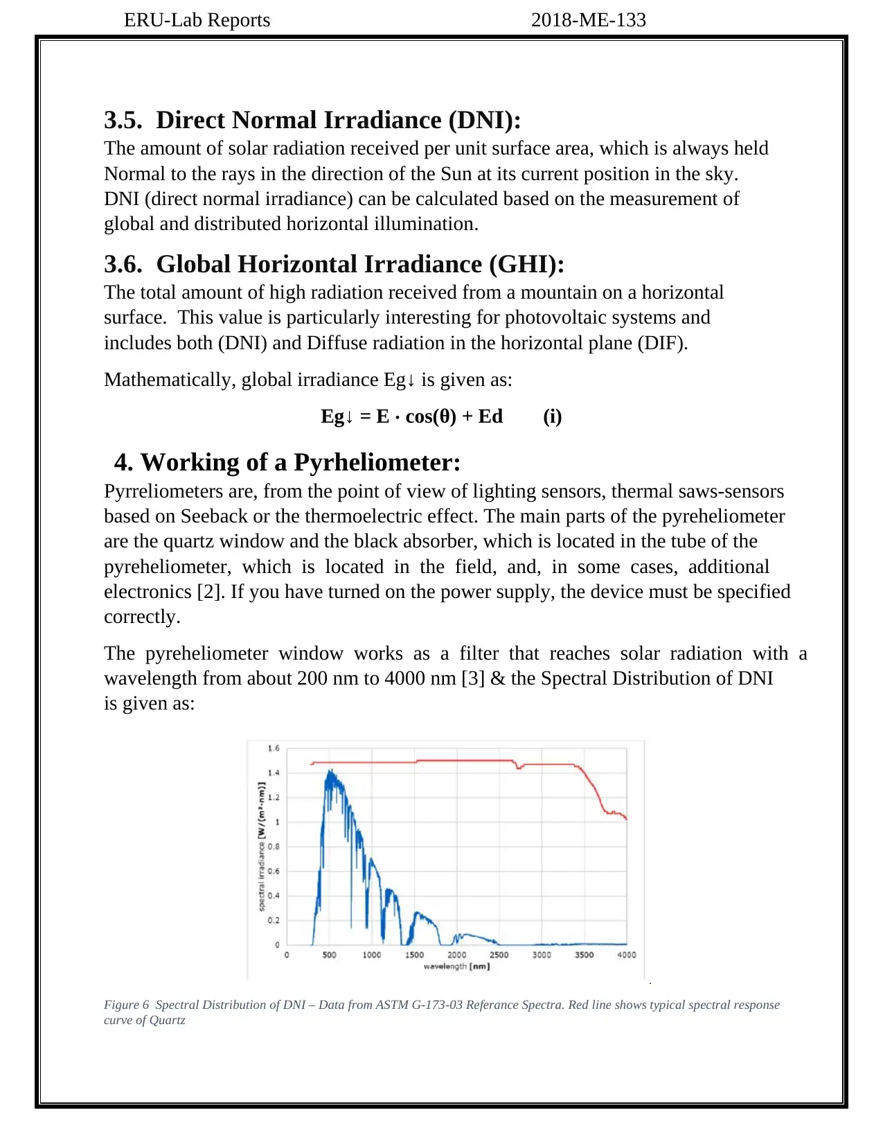
3.3. Pyrheliometer a Solar Irriadiance Sensor:
Pyreheliometers measure direct solar radiation, this is also known as direct normal
solar radiation, often transcribed as DNI.
Pyreheliometer must be installed on a solar tracker: a device in which aspects of
the device are exposed to the sun during the day[1]. The total amount of available
solar energy on the earth's surface on a decreasing scale of solar radiation Eg↓ is
given Mathematically as:
Eg↓ = E ⋅ cos(θ) + Ed
Figure 5 Pyrometers measure Direct Solar radiation
3.4. Difference between Pyrheliometer & Pyranometer:
Both the instruments like Pyrheliometer & Pyranometer are used to calculate solar
irradiance. These are related in their intention but there are some dissimilarities in
their construction & working principle.
Pyranometer Pyrhellometer
It is one kind of acidometer mainly used to
measure the solar irradiance over a planner
surface
It is used to measure direct ray solar irradiance
It utilizes the principle of thermoelectric
detection.
It also uses the thermoelectric detection
principle.
In this, the measurement of increasing
temperature can be done through
thermocouples and they are linked in series.
It this the increasing temperature can be
calculated through thermocouples which are
allied in series.
The instrument calculated global solar
radiation
This instrument is used to find the direct solar
radiation.
Paraphrase This Document
Need a fresh take? Get an instant paraphrase of this document with our AI Paraphraser
ERU-Lab Reports 2018-ME-133
3.5. Direct Normal Irradiance (DNI):
The amount of solar radiation received per unit surface area, which is always held
Normal to the rays in the direction of the Sun at its current position in the sky.
DNI (direct normal irradiance) can be calculated based on the measurement of
global and distributed horizontal illumination.
3.6. Global Horizontal Irradiance (GHI):
The total amount of high radiation received from a mountain on a horizontal
surface. This value is particularly interesting for photovoltaic systems and
includes both (DNI) and Diffuse radiation in the horizontal plane (DIF).
Mathematically, global irradiance Eg↓ is given as:
Eg↓ = E ⋅ cos(θ) + Ed (i)
4. Working of a Pyrheliometer:
Pyrreliometers are, from the point of view of lighting sensors, thermal saws-sensors
based on Seeback or the thermoelectric effect. The main parts of the pyreheliometer
are the quartz window and the black absorber, which is located in the tube of the
pyreheliometer, which is located in the field, and, in some cases, additional
electronics [2]. If you have turned on the power supply, the device must be specified
correctly.
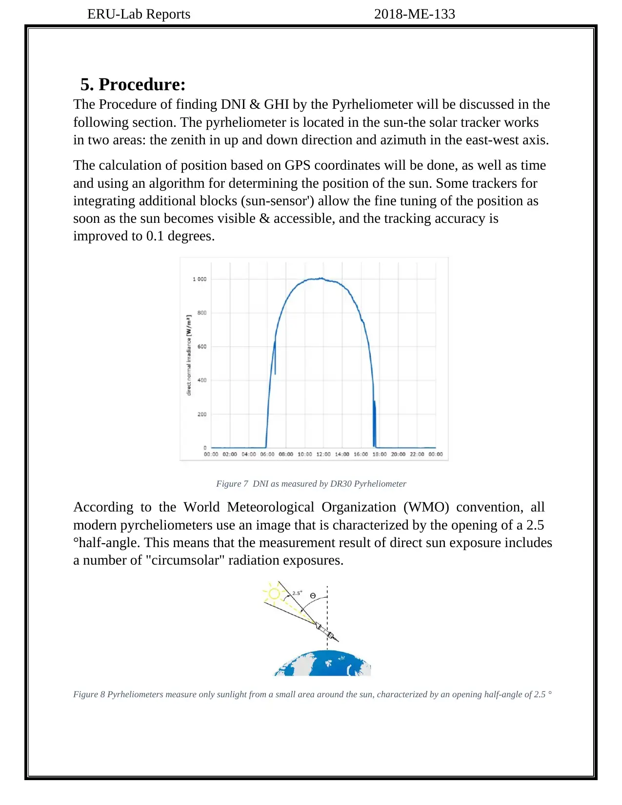
The pyreheliometer window works as a filter that reaches solar radiation with a
wavelength from about 200 nm to 4000 nm [3] & the Spectral Distribution of DNI
is given as:
Figure 6 Spectral Distribution of DNI – Data from ASTM G-173-03 Referance Spectra. Red line shows typical spectral response
curve of Quartz
3.5. Direct Normal Irradiance (DNI):
The amount of solar radiation received per unit surface area, which is always held
Normal to the rays in the direction of the Sun at its current position in the sky.
DNI (direct normal irradiance) can be calculated based on the measurement of
global and distributed horizontal illumination.
3.6. Global Horizontal Irradiance (GHI):
The total amount of high radiation received from a mountain on a horizontal
surface. This value is particularly interesting for photovoltaic systems and
includes both (DNI) and Diffuse radiation in the horizontal plane (DIF).
Mathematically, global irradiance Eg↓ is given as:
Eg↓ = E ⋅ cos(θ) + Ed (i)
4. Working of a Pyrheliometer:
Pyrreliometers are, from the point of view of lighting sensors, thermal saws-sensors
based on Seeback or the thermoelectric effect. The main parts of the pyreheliometer
are the quartz window and the black absorber, which is located in the tube of the
pyreheliometer, which is located in the field, and, in some cases, additional
electronics [2]. If you have turned on the power supply, the device must be specified
correctly.
The pyreheliometer window works as a filter that reaches solar radiation with a
wavelength from about 200 nm to 4000 nm [3] & the Spectral Distribution of DNI
is given as:
Figure 6 Spectral Distribution of DNI – Data from ASTM G-173-03 Referance Spectra. Red line shows typical spectral response
curve of Quartz
ERU-Lab Reports 2018-ME-133
5. Procedure:
The Procedure of finding DNI & GHI by the Pyrheliometer will be discussed in the
following section. The pyrheliometer is located in the sun-the solar tracker works
in two areas: the zenith in up and down direction and azimuth in the east-west axis.
The calculation of position based on GPS coordinates will be done, as well as time
and using an algorithm for determining the position of the sun. Some trackers for
integrating additional blocks (sun-sensor') allow the fine tuning of the position as
soon as the sun becomes visible & accessible, and the tracking accuracy is
improved to 0.1 degrees.
Figure 7 DNI as measured by DR30 Pyrheliometer
According to the World Meteorological Organization (WMO) convention, all
modern pyrcheliometers use an image that is characterized by the opening of a 2.5
°half-angle. This means that the measurement result of direct sun exposure includes
a number of "circumsolar" radiation exposures.
Figure 8 Pyrheliometers measure only sunlight from a small area around the sun, characterized by an opening half-angle of 2.5 °
⊘ This is a preview!⊘
Do you want full access?
Subscribe today to unlock all pages.
Trusted by 1+ million students worldwide
1 out of 71
Your All-in-One AI-Powered Toolkit for Academic Success.
+13062052269
info@desklib.com
Available 24*7 on WhatsApp / Email
![[object Object]](/_next/static/media/star-bottom.7253800d.svg)
Unlock your academic potential
Copyright © 2020–2026 A2Z Services. All Rights Reserved. Developed and managed by ZUCOL.