Exploring Bayes-Nash Equilibrium in Game Theory: Bertrand Pricing

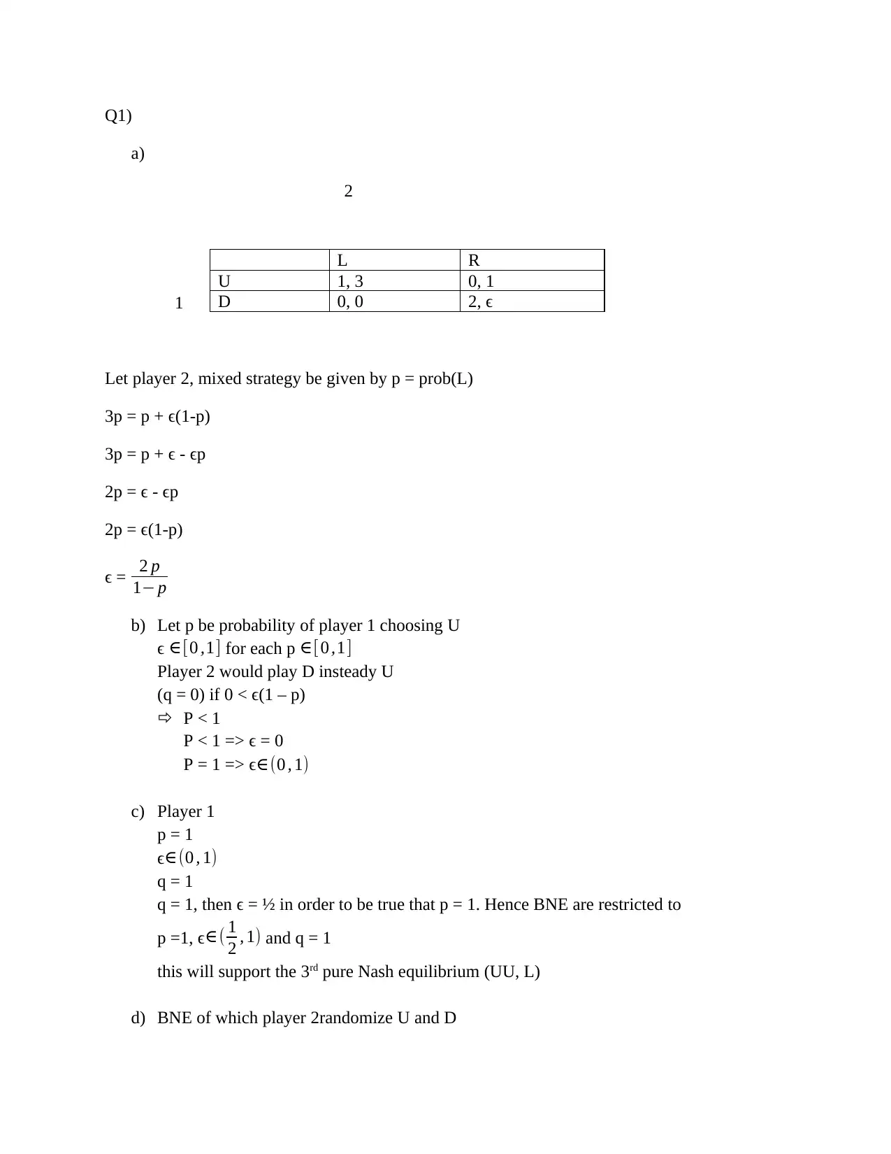
This assignment delves into the concept of Bayes-Nash equilibrium within the context of game theory, specifically focusing on its application to Bertrand pricing games. It explores mixed strategies, analyzes the conditions for equilibrium, and examines scenarios with varying information and player types. The solutions cover problems related to the determination of Bayes-Nash equilibria in different scenarios, including cases where players randomize their strategies. The assignment also addresses the impact of cost parameters on firms' production decisions and the existence of pure strategy Bayes-Nash equilibria. This detailed exploration provides a comprehensive understanding of strategic interactions in economic models, offering valuable insights for students studying game theory. Desklib provides a platform to explore similar solved assignments and past papers.

Q1)
a)
2
1
Let player 2, mixed strategy be given by p = prob(L)
3p = p + ϵ(1-p)
3p = p + ϵ - ϵp
2p = ϵ - ϵp
2p = ϵ(1-p)
ϵ = 2 p
1− p
b) Let p be probability of player 1 choosing U
ϵ ∈[0 ,1] for each p ∈[ 0 ,1]
Player 2 would play D insteady U
(q = 0) if 0 < ϵ(1 – p)
 P < 1
P < 1 => ϵ = 0
P = 1 => ϵ∈(0 , 1)
c) Player 1
p = 1
ϵ∈(0 , 1)
q = 1
q = 1, then ϵ = ½ in order to be true that p = 1. Hence BNE are restricted to
p =1, ϵ∈( 1
2 , 1) and q = 1
this will support the 3rd pure Nash equilibrium (UU, L)
d) BNE of which player 2randomize U and D
L R
U 1, 3 0, 1
D 0, 0 2, ϵ

Player 2 plays L
Player 2 plays L in steady of R
R(p =1) if ½ [3q + 0(1-q)] > ½ [1q + ϵ(1-q)]
3/2q > ½ [q + ϵ - ϵq]
3/2q – 1/2q > ½ ϵ(1 –q)
q > ½ ϵ(1-q)
this can be summarized as
q > ½ ∈ (1−q )=¿ p=1
q = 1 => ϵ ∈ [ 0 , 1 ]
Q2
20.14 Find at least one mixed – strategy Bayes – Nash equilibrium in the Bertrand pricing game
First mixed strategy
Suppose the husband plays F with probability 1. A type 1 wife’s expected payoff from playing F
is therefore 1
Playing O is 3(1, -1). The wife plays a mixed strategy only if she were indifferent between F and
O, that is, if λ -3(1-λ) or λ = ¾
Second mixed strategy
Type 2 wife would get the same payoffs from playing F as type 1 wife gets from playing O,
similarly same payoffs would play O as a type 1 wife gets from playing F
Third mixed strategy
The husband would be indifferent only when; 3μ1ρ + 3μ2(1 -ρ ¿ = (1 - μ1)ρ+1−μ2)(1- ρ ¿,
therefore F and O would be best responses, therefore, λ = ¾ would be best response
Fourth mixed strategy
If mixed strategies (m1, m2) would satisfy ρ ( 4 μ 1−1 ) =(1−ρ)(1−4 μ 2), the husband would
have best mixed strategy response of λ = ¾
Fifth mixed strategy
When the husband would play λ = ¾ then mixed strategy pair (m1, m2) would be best response
for the wives

20.15
Regardless of r value, there must be a mixed strategy Bayes Nash equilibrium when;
λ = ¾, μ1, μ2 = (1/4, ¼)
Any addition mixed strategy Bayes Nash equilibrium would characterized by λ = ¾ and (m1,
m2) should satisfy ρ ( 4 μ 1−1 ) =(1−ρ)¿)
20.16
Two pure strategies Bayes Nash equilibrium would exist whenρ> 3
4 . When the husband F and
wives play (F, O) in the first case. The second case is when the husband would play O and wives
would play (O, F). One pure strategy Bayes Nash equilibrium would exist when ¼ ≤ ρ< 3
4
20.17
If ρ< 1
4 , then r =0, where the husband knows that her wife is type 2. There would be no pure
strategy Nash equilibrium. Since the husband wants to go to a same event but the wife wants to
go to a different event.
20.18
Probability of of husband playing F = 1
The expected playoff of wife type 1 playing F = 1
Type 1 wife playing O the playoff = 3(1 -1)
Mixed strategy that would be played by the wife if she would be indifferent between F and O
would be when λ-3(1-λ) or when λ = ¾
Type 2 would get the same payoff as she play F while type 1 would be playing O, similarly when
type 2 would play O she would get the same playoff while type 1 wife plays F
20.19

a) Type 2 wife would require a probability of 1 – r who plays F having probability m2
The husband playoff would be equal to 3 and would play O at a probability of 1 – m2 that would
yield a pay of 0
The husband expects a payoff when he plays O
The husband would prefer F to O if 3μ1ρ + 3μ2(1 - ρ ¿ > (1 - μ1)ρ+1−μ2)(1-ρ ¿
The husband would be indifferent if 3μ1 ρ + 3μ2(1 - ρ ¿ = (1 - μ1) ρ+1−μ2)(1- ρ ¿
The best response would be λ = ¾
b) Regardless of r value, there must be a mixed strategy Bayes Nash equilibrium when;
λ = ¾, μ1, μ2 = (1/4, ¼)
20.20
Provided provide with probability r, type 1 wife who would be playing F would be met by the
husband, having a probability m1
The husband playoff = 3 and play O at a probability of 1 – m1.
Meeting type 2 wife would require a probability of 1 – r who plays F having probability m2
The husband playoff would be equal to 3 and would play O at a probability of 1 – m2 that would
yield a pay of 0
The husband expects a payoff when he plays O
The husband would prefer F to O if 3μ1 ρ + 3μ2(1 - ρ ¿ > (1 - μ1) ρ+1−μ2)(1- ρ ¿
The husband would be indifferent if 3μ1ρ + 3μ2(1 - ρ ¿ = (1 - μ1)ρ+1−μ2)(1-ρ ¿
The best response would be λ = ¾
20.21
The husband expects a payoff when he plays O
The husband would prefer F to O if 3μ1ρ + 3μ2(1 - ρ ¿ > (1 - μ1)ρ+1−μ2)(1-ρ ¿
The husband would be indifferent if 3μ1 ρ + 3μ2(1 - ρ ¿ = (1 - μ1) ρ+1−μ2)(1- ρ ¿
The best response would be λ = ¾
20.22
q1 = loving wives

q2 = leaving wives
H/W Type 1 Type 2
Type 1 q * ρ q *(1- ρ)
Type 2 (1 –q) * ρ (1 –q) *¿)
Type 1 wife probability = qp
q ρ+(1−q) ρ for q1
Type 2 wife probability = q (1−ρ)
q ( 1−ρ )−(1−q)(1− ρ) for q2
20.23
At q = 1/2 , ρ= 3
4 and ρ= 3
4
Then ,
Type 1 wife probability = qp
q ρ+(1−q) ρ for q1
Type 2 wife probability = q (1−ρ)
q ( 1−ρ )−(1−q)(1− ρ) for q2
The husbands would play both F and O, while the wives would play O and F simultaneously.
20.24
Yes, the addition pure strategy Bayes equilibria that would exist would be characterized by λ = ¾
and (m1, m2) that would satisfy ρ ( 4 μ 1−1 )=(1−ρ)¿ equation
21.1
Cournot competition firms
They compete over quantity
If firm 1 do not know firm 2 cost, while firm 1 has a marginal cost, which would be taken as the
cost of producing quantity Q1 = cQ1

Firm 2 having too marginal cost that is constant, and the marginal cost is only known to firm 2
owners, the marginal cost would be c + `I
The `I would range between –X and X having a mean of zero
Therefore. The marginal cost of firm 2 would be different from firm 1
If the marginal cost of firm c ids less than c
The outcome would occur when `I ≪ 0
If the marginal cost of firm 2 would be greater than c the outcome would be `I > 0
Bertrand completion firms
They compete over price
21.2
The cost parameter `I when it would be higher, it would mean that firm 2 would have less cost to
produce best responses
An `I that would be non-average would produce lass baseline if `I >0, while at lower cost it would
produce more products than the average at `I ≪ 0
21.3
Firm 1
Maximum profit from first order condition =
10−ϵ−1−Q 2
Firm 2
Total cost = (c + `I ¿ Q 2
Profit maximizing quantity would be
max
q 2 ≥0
[10−ϵ− ( Q 1+Q 2 ) ] Q2
Maximum profit quantity from first order

10−ϵ−Q 1−2 Q2 =0
Q2 = 10−ϵ −Q1
2
21.4
Firm 2
Total cost = (c + `I ¿ Q 2
Profit maximizing quantity would be
max
q 2 ≥0
[10−ϵ− ( Q 1+Q 2 ) ] Q2
Where
eQ2 `I is the expected firm 2 quantity that it will produce
Maximum profit quantity from first order
10−ϵ−Q 1−2 Q2 =0
Q2 = 10−ϵ −Q1
2
eQ2 `I = e [ 10−ϵ−Q 1
2 ]
= 2 [ 10−ϵ −Q1
2 ]
= 10−ϵ−Q 1
When firm 2 costs are high the profit equilibrium of 1 would be highest, firm 2 profits would be
high at `I = -X and would decrease to highest cost of `I = X
21.5
Total cost = (c + `I ¿ Q 2

Profit maximizing quantity would be
max
q 2 ≥0
[10−ϵ− ( Q 1+Q 2 ) ] Q2
Maximum profit quantity from first order
10−ϵ−Q 1−2 Q2 =0
Q2 = 10−ϵ −Q1
2
Therefore,
Q1 = 10−ϵ −2Q 2
R1 Q2 = {10−ϵ−Q 1
2 if Q 1≤ 10−ϵ
0if Q 1 ≥10−ϵ
21.6
The conjectures would coincide at Q1*, Q2*(ϵ) having best responses. This would mean that
Q2*(ϵ) amount that a firm one would conjectures `I type of firm 2 that it would produce would be
equivalent types of production that is equivalent to R1 Q1*(ϵ) for firm 1 average conjecture
21.7
Maximum profit quantity from first order
10−ϵ−Q 1−2 Q2 =0
Q1 = 10−ϵ −Q2
2
Best response would be
R1(Q2) = 10−ϵ −Q1
2
21.8

Quantity produced in the market = 10−ϵ −Q1
2
Average price = c = marginal cost