Data Analysis of TfL Santander Bike Hire Scheme - QUA4A5 Project
VerifiedAdded on 2022/08/26
|12
|2120
|16
Project
AI Summary
This project, undertaken as part of the QUA4A5 course, analyzes a dataset of Transport for London's (TfL) Santander Bike Hire Scheme. The analysis investigates bike hire trends, including daily and seasonal variations, and the correlation between daily temperature and the number of bike hires. The project utilizes MS Excel for statistical calculations, including mean, median, standard deviation, and confidence intervals, as well as forecasting techniques to predict bike usage. The project also explores data distribution, random sampling, and regression analysis to determine the relationship between temperature and bike hires, with two regression models developed and compared. The findings reveal insights into bike hire patterns and the influence of external factors, providing recommendations for optimizing the scheme's operations.

QUA4A5 Assessment 3: Group Project
TfL Case study assignment
Name of the Student
Name of the University
TfL Case study assignment
Name of the Student
Name of the University
Paraphrase This Document
Need a fresh take? Get an instant paraphrase of this document with our AI Paraphraser
Table of Contents
Introduction................................................................................................................................3
Task I..........................................................................................................................................3
Part [a]....................................................................................................................................3
Part [b]....................................................................................................................................3
Part [c]....................................................................................................................................4
Task II........................................................................................................................................5
Part [a]....................................................................................................................................5
Part [b]....................................................................................................................................5
Task III.......................................................................................................................................5
Part [a]....................................................................................................................................5
Part [b]....................................................................................................................................6
Task IV.......................................................................................................................................7
Part [a]....................................................................................................................................7
Part [b]....................................................................................................................................8
Task V........................................................................................................................................9
Part [a]....................................................................................................................................9
Part [b]....................................................................................................................................9
Part [c]..................................................................................................................................10
Conclusion................................................................................................................................10
Reference..................................................................................................................................11
Introduction
The aim of this project is to evaluate a large data gathered by Transport for London's (TfL's)
related to their 'Santander' Bike Hire Scheme. In specific, in this project work, being the
director of TfL, the author tried to investigate number of bike hires on each day, each season,
the general trend and any association between daily temperature and number of bike hires.
The entire investigation has been divided in 5 sub tasks that are mentioned in the subsequent
section. The author at the same time used MS excel function to predict 7 days possible
number of bikes hiring.
Task I
Part [a]
In this section, the author has calculated mean, median and standard deviation of daily bike
hire based on historical data. The table below is showing the details:
Mean 31705.8
Median 33112
Sample Stdev 11300.3
Standard Error of Mean 292.583
Z95% 1.96
Lower confidence Limit 31132.3
Upper confidence Limit 32279.2
Table 1: mean, median, std dev, confidence interval
[Source: calculation done in excel]
The above table is also showing the 95% confidence interval of population mean of daily
bike hiring. From the above table, it can be concluded that on an average daily basis 31706
bikes were hired from different places in London. At the same time, this table is also
indicating that 50% cases the number of bikes hired on daily basis was more than 33112.
Based on this sample data, the author further concluded that there is a 95% chance that in any
days the number of bikes will be hired will remain in between 31132 to 32279.
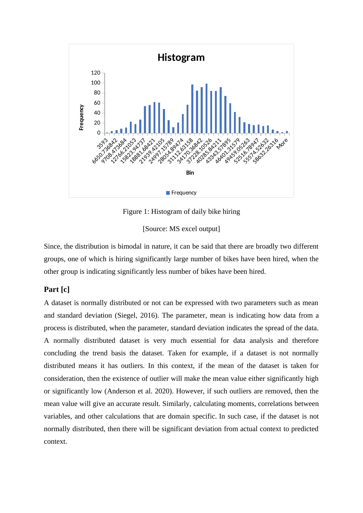
Part [b]
The sample data set related to number of bicycles hiring is not normally distributed. Rather,
with reference to the histogram mentioned below, it can be concluded that the sample is
following a bimodal distribution.
The aim of this project is to evaluate a large data gathered by Transport for London's (TfL's)
related to their 'Santander' Bike Hire Scheme. In specific, in this project work, being the
director of TfL, the author tried to investigate number of bike hires on each day, each season,
the general trend and any association between daily temperature and number of bike hires.
The entire investigation has been divided in 5 sub tasks that are mentioned in the subsequent
section. The author at the same time used MS excel function to predict 7 days possible
number of bikes hiring.
Task I
Part [a]
In this section, the author has calculated mean, median and standard deviation of daily bike
hire based on historical data. The table below is showing the details:
Mean 31705.8
Median 33112
Sample Stdev 11300.3
Standard Error of Mean 292.583
Z95% 1.96
Lower confidence Limit 31132.3
Upper confidence Limit 32279.2
Table 1: mean, median, std dev, confidence interval
[Source: calculation done in excel]
The above table is also showing the 95% confidence interval of population mean of daily
bike hiring. From the above table, it can be concluded that on an average daily basis 31706
bikes were hired from different places in London. At the same time, this table is also
indicating that 50% cases the number of bikes hired on daily basis was more than 33112.
Based on this sample data, the author further concluded that there is a 95% chance that in any
days the number of bikes will be hired will remain in between 31132 to 32279.
Part [b]
The sample data set related to number of bicycles hiring is not normally distributed. Rather,
with reference to the histogram mentioned below, it can be concluded that the sample is
following a bimodal distribution.
⊘ This is a preview!⊘
Do you want full access?
Subscribe today to unlock all pages.
Trusted by 1+ million students worldwide
3593
6650.736842
9708.473684
12766.21053
15823.94737
18881.68421
21939.42105
24997.15789
28054.89474
31112.63158
34170.36842
37228.10526
40285.84211
43343.57895
46401.31579
49459.05263
52516.78947
55574.52632
58632.26316
More
0
20
40
60
80
100
120
Histogram
Frequency
Bin
Frequency
Figure 1: Histogram of daily bike hiring
[Source: MS excel output]
Since, the distribution is bimodal in nature, it can be said that there are broadly two different
groups, one of which is hiring significantly large number of bikes have been hired, when the
other group is indicating significantly less number of bikes have been hired.
Part [c]
A dataset is normally distributed or not can be expressed with two parameters such as mean
and standard deviation (Siegel, 2016). The parameter, mean is indicating how data from a
process is distributed, when the parameter, standard deviation indicates the spread of the data.
A normally distributed dataset is very much essential for data analysis and therefore
concluding the trend basis the dataset. Taken for example, if a dataset is not normally
distributed means it has outliers. In this context, if the mean of the dataset is taken for
consideration, then the existence of outlier will make the mean value either significantly high
or significantly low (Anderson et al. 2020). However, if such outliers are removed, then the
mean value will give an accurate result. Similarly, calculating moments, correlations between
variables, and other calculations that are domain specific. In such case, if the dataset is not
normally distributed, then there will be significant deviation from actual context to predicted
context.
Paraphrase This Document
Need a fresh take? Get an instant paraphrase of this document with our AI Paraphraser
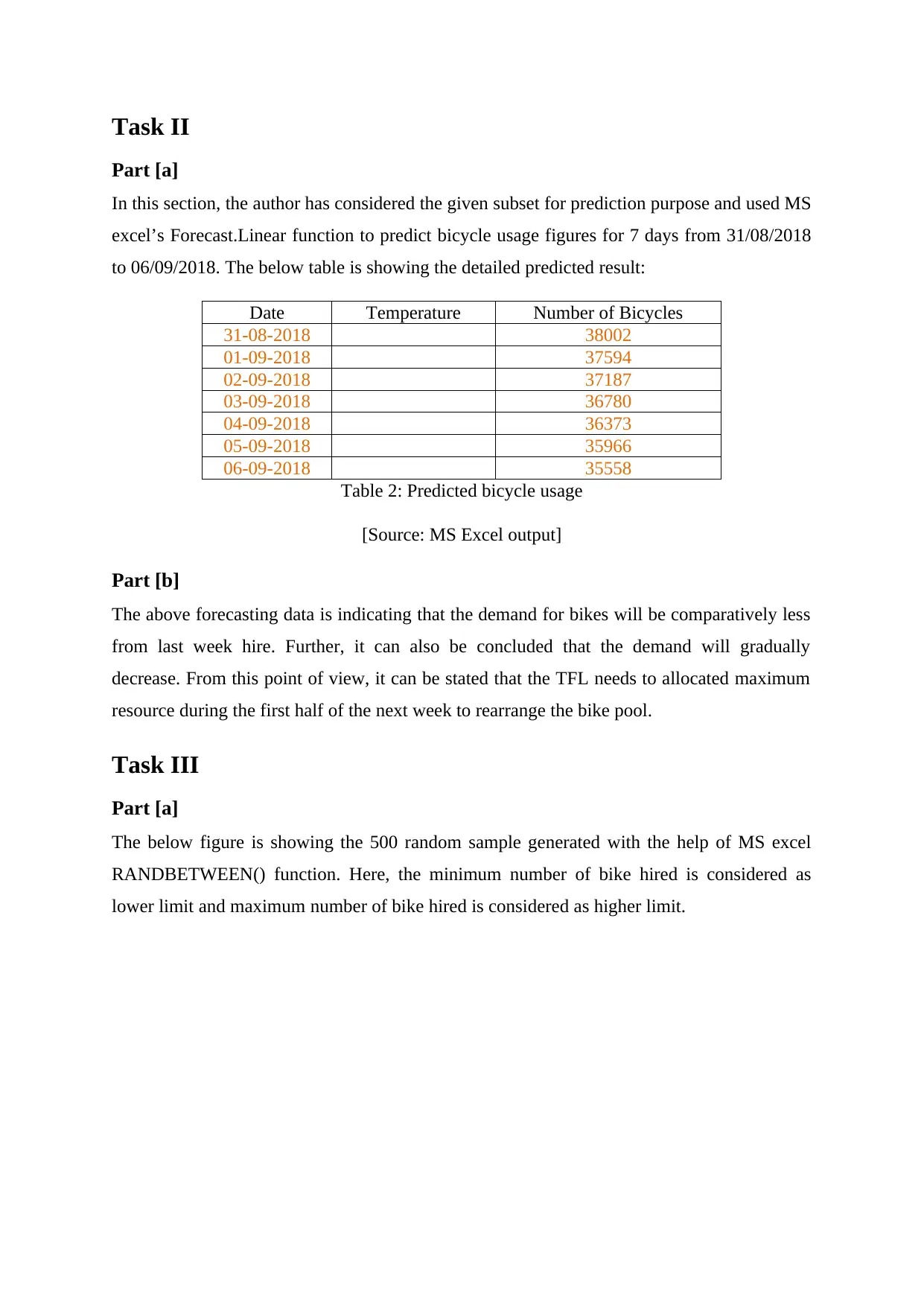
Task II
Part [a]
In this section, the author has considered the given subset for prediction purpose and used MS
excel’s Forecast.Linear function to predict bicycle usage figures for 7 days from 31/08/2018
to 06/09/2018. The below table is showing the detailed predicted result:
Date Temperature Number of Bicycles
31-08-2018 38002
01-09-2018 37594
02-09-2018 37187
03-09-2018 36780
04-09-2018 36373
05-09-2018 35966
06-09-2018 35558
Table 2: Predicted bicycle usage
[Source: MS Excel output]
Part [b]
The above forecasting data is indicating that the demand for bikes will be comparatively less
from last week hire. Further, it can also be concluded that the demand will gradually
decrease. From this point of view, it can be stated that the TFL needs to allocated maximum
resource during the first half of the next week to rearrange the bike pool.
Task III
Part [a]
The below figure is showing the 500 random sample generated with the help of MS excel
RANDBETWEEN() function. Here, the minimum number of bike hired is considered as
lower limit and maximum number of bike hired is considered as higher limit.
Part [a]
In this section, the author has considered the given subset for prediction purpose and used MS
excel’s Forecast.Linear function to predict bicycle usage figures for 7 days from 31/08/2018
to 06/09/2018. The below table is showing the detailed predicted result:
Date Temperature Number of Bicycles
31-08-2018 38002
01-09-2018 37594
02-09-2018 37187
03-09-2018 36780
04-09-2018 36373
05-09-2018 35966
06-09-2018 35558
Table 2: Predicted bicycle usage
[Source: MS Excel output]
Part [b]
The above forecasting data is indicating that the demand for bikes will be comparatively less
from last week hire. Further, it can also be concluded that the demand will gradually
decrease. From this point of view, it can be stated that the TFL needs to allocated maximum
resource during the first half of the next week to rearrange the bike pool.
Task III
Part [a]
The below figure is showing the 500 random sample generated with the help of MS excel
RANDBETWEEN() function. Here, the minimum number of bike hired is considered as
lower limit and maximum number of bike hired is considered as higher limit.
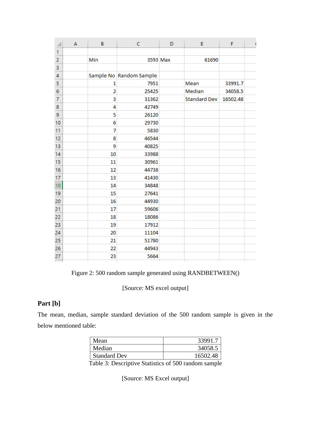
Figure 2: 500 random sample generated using RANDBETWEEN()
[Source: MS excel output]
Part [b]
The mean, median, sample standard deviation of the 500 random sample is given in the
below mentioned table:
Mean 33991.7
Median 34058.5
Standard Dev 16502.48
Table 3: Descriptive Statistics of 500 random sample
[Source: MS Excel output]
[Source: MS excel output]
Part [b]
The mean, median, sample standard deviation of the 500 random sample is given in the
below mentioned table:
Mean 33991.7
Median 34058.5
Standard Dev 16502.48
Table 3: Descriptive Statistics of 500 random sample
[Source: MS Excel output]
⊘ This is a preview!⊘
Do you want full access?
Subscribe today to unlock all pages.
Trusted by 1+ million students worldwide
The mean of given data set is 31706 when the mean of 500 random sample is 33992. It
means, the random sample is showing comparatively higher hiring forecast than the actual
figure. The median and standard deviation results also supporting the same conclusion.
Task IV
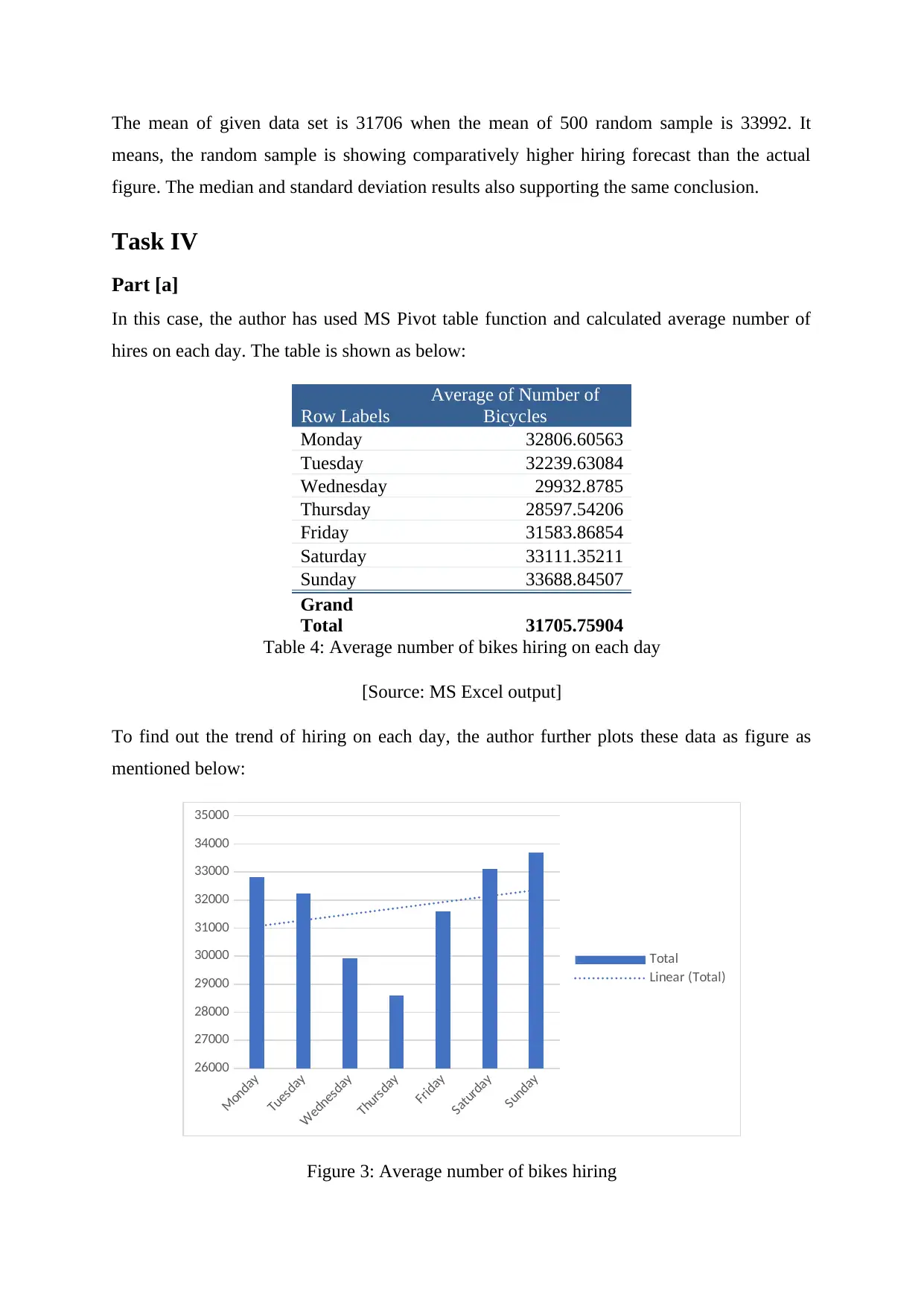
Part [a]
In this case, the author has used MS Pivot table function and calculated average number of
hires on each day. The table is shown as below:
Row Labels
Average of Number of
Bicycles
Monday 32806.60563
Tuesday 32239.63084
Wednesday 29932.8785
Thursday 28597.54206
Friday 31583.86854
Saturday 33111.35211
Sunday 33688.84507
Grand
Total 31705.75904
Table 4: Average number of bikes hiring on each day
[Source: MS Excel output]
To find out the trend of hiring on each day, the author further plots these data as figure as
mentioned below:
Monday
Tuesday
Wednesday
Thursday
Friday
Saturday
Sunday
26000
27000
28000
29000
30000
31000
32000
33000
34000
35000
Total
Linear (Total)
Figure 3: Average number of bikes hiring
means, the random sample is showing comparatively higher hiring forecast than the actual
figure. The median and standard deviation results also supporting the same conclusion.
Task IV
Part [a]
In this case, the author has used MS Pivot table function and calculated average number of
hires on each day. The table is shown as below:
Row Labels
Average of Number of
Bicycles
Monday 32806.60563
Tuesday 32239.63084
Wednesday 29932.8785
Thursday 28597.54206
Friday 31583.86854
Saturday 33111.35211
Sunday 33688.84507
Grand
Total 31705.75904
Table 4: Average number of bikes hiring on each day
[Source: MS Excel output]
To find out the trend of hiring on each day, the author further plots these data as figure as
mentioned below:
Monday
Tuesday
Wednesday
Thursday
Friday
Saturday
Sunday
26000
27000
28000
29000
30000
31000
32000
33000
34000
35000
Total
Linear (Total)
Figure 3: Average number of bikes hiring
Paraphrase This Document
Need a fresh take? Get an instant paraphrase of this document with our AI Paraphraser
[Source: MS excel output]
It is clear that the maximum number of hiring happened during the start and end of the week.
Overall, there is a linear upward trend of hiring, which means, the maximum number of
hiring happened on Sundays and Saturdays. The lowest number of hiring happened on
Thursday.
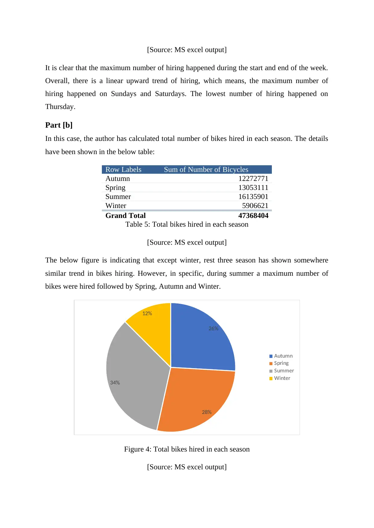
Part [b]
In this case, the author has calculated total number of bikes hired in each season. The details
have been shown in the below table:
Row Labels Sum of Number of Bicycles
Autumn 12272771
Spring 13053111
Summer 16135901
Winter 5906621
Grand Total 47368404
Table 5: Total bikes hired in each season
[Source: MS excel output]
The below figure is indicating that except winter, rest three season has shown somewhere
similar trend in bikes hiring. However, in specific, during summer a maximum number of
bikes were hired followed by Spring, Autumn and Winter.
26%
28%
34%
12%
Autumn
Spring
Summer
Winter
Figure 4: Total bikes hired in each season
[Source: MS excel output]
It is clear that the maximum number of hiring happened during the start and end of the week.
Overall, there is a linear upward trend of hiring, which means, the maximum number of
hiring happened on Sundays and Saturdays. The lowest number of hiring happened on
Thursday.
Part [b]
In this case, the author has calculated total number of bikes hired in each season. The details
have been shown in the below table:
Row Labels Sum of Number of Bicycles
Autumn 12272771
Spring 13053111
Summer 16135901
Winter 5906621
Grand Total 47368404
Table 5: Total bikes hired in each season
[Source: MS excel output]
The below figure is indicating that except winter, rest three season has shown somewhere
similar trend in bikes hiring. However, in specific, during summer a maximum number of
bikes were hired followed by Spring, Autumn and Winter.
26%
28%
34%
12%
Autumn
Spring
Summer
Winter
Figure 4: Total bikes hired in each season
[Source: MS excel output]
Task V
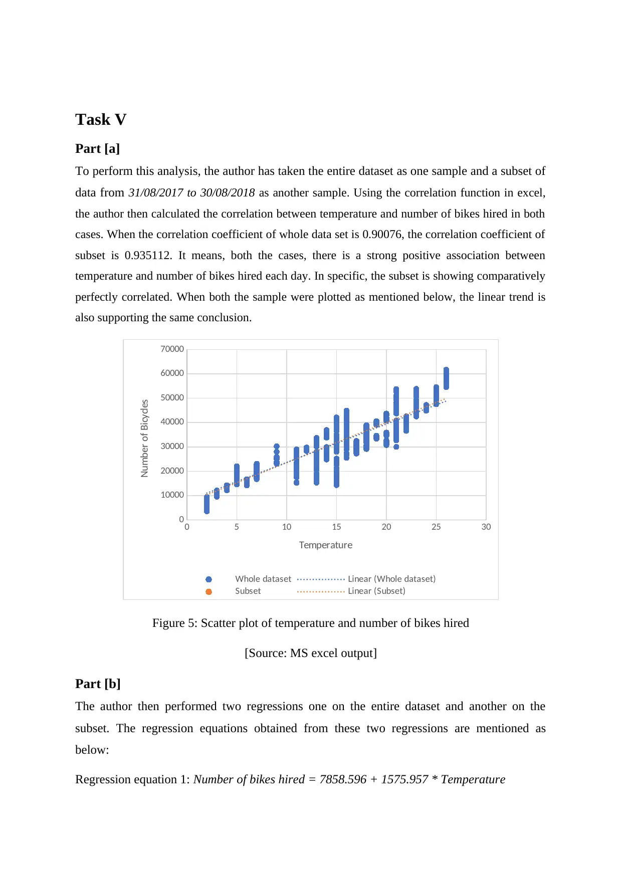
Part [a]
To perform this analysis, the author has taken the entire dataset as one sample and a subset of
data from 31/08/2017 to 30/08/2018 as another sample. Using the correlation function in excel,
the author then calculated the correlation between temperature and number of bikes hired in both
cases. When the correlation coefficient of whole data set is 0.90076, the correlation coefficient of
subset is 0.935112. It means, both the cases, there is a strong positive association between
temperature and number of bikes hired each day. In specific, the subset is showing comparatively
perfectly correlated. When both the sample were plotted as mentioned below, the linear trend is
also supporting the same conclusion.
0 5 10 15 20 25 30
0
10000
20000
30000
40000
50000
60000
70000
Whole dataset Linear (Whole dataset)
Subset Linear (Subset)
Temperature
Number of Bicycles
Figure 5: Scatter plot of temperature and number of bikes hired
[Source: MS excel output]
Part [b]
The author then performed two regressions one on the entire dataset and another on the
subset. The regression equations obtained from these two regressions are mentioned as
below:
Regression equation 1: Number of bikes hired = 7858.596 + 1575.957 * Temperature
⊘ This is a preview!⊘
Do you want full access?
Subscribe today to unlock all pages.
Trusted by 1+ million students worldwide
Regression equation 2: Number of bikes hired = 7027.83 + 1649.676 * Temperature
From these two equations, it can be concluded that if temperature is become 0, then
regression equation 1 will give 7859 hiring instances, when regression equation 2 will give
7028 hiring. However, as the temperature goes high, regression equation 2 will give better
number of hiring.
The R^2 value indicates the degree of accuracy of the regression equation developed in the
above section (Black, 2019). From regression equation 1, the R^2 value is 81.1368% when
the regression equation 2 is showing 87.4435%. It means, there will be 87.4435% chance that
regression equation 2 will give accurate result, when 81.1368% chance that regression
equation 1 will give accurate result.
The F value is the ratio of the mean regression sum of squares divided by the mean error
sum of squares (Anderson et al. 2020). Its value will range from zero to an arbitrarily large
number (Jaggia et al. 2016). The value of Prob(F) is the probability that the null hypothesis
for the full model is true (i.e., that all of the regression coefficients are zero) (Robertson, and
McCloskey, 2019). In case of regression 1, F statistic is comparatively high than regression 2.
In case of probability value, both are less than 0.05, which means both the model can be
applied to predict number of bikes hiring basis the temperature on each day (Geis, 2019).
Considering all the values, regression equation results, it can be concluded that second
regression is describing the data better.
Part [c]
The above section has shown that temperature is a major factor behind predicting number of
bikes hired on each day. However, the same kind of observation could have obtained
considering season as another important factor. Apart from this, location wise data might
have given another view and accordingly TfL can conclude which suburb is giving maximum
hiring and all.
Conclusion
Thus, to conclude it can be said that the given data set has helped to find out an overall trend
of bike hiring especially basis the temperature. However, the data is all about seasonal
details. The TfL could have gathered other essential information along with existing data to
make prediction in a better way.
Paraphrase This Document
Need a fresh take? Get an instant paraphrase of this document with our AI Paraphraser


Reference
Anderson, D.R., Sweeney, D.J., Williams, T.A., Camm, J.D. and Cochran, J.J., 2020.
Modern business statistics with Microsoft Excel. Cengage Learning.
Anderson, D.R., Sweeney, D.J., Williams, T.A., Camm, J.D. and Cochran, J.J., 2020.
Essentials of modern business statistics with Microsoft Excel. Cengage Learning.
Black, K., 2019. Business statistics: for contemporary decision making. John Wiley & Sons.
Geis, G.T., 2019. Business Statistics. Thomson Publishing Company.
Jaggia, S., Kelly, A., Salzman, S., Olaru, D., Sriananthakumar, S., Beg, R. and Leighton, C.,
2016. Essentials of Business Statistics: communicating with numbers. McGrawhill Education.
Robertson, C. and McCloskey, M., 2019. Business Statistics A multimedia guide to concepts
and applications. Oxford University Press.
Siegel, A., 2016. Practical business statistics. Academic Press.
Anderson, D.R., Sweeney, D.J., Williams, T.A., Camm, J.D. and Cochran, J.J., 2020.
Modern business statistics with Microsoft Excel. Cengage Learning.
Anderson, D.R., Sweeney, D.J., Williams, T.A., Camm, J.D. and Cochran, J.J., 2020.
Essentials of modern business statistics with Microsoft Excel. Cengage Learning.
Black, K., 2019. Business statistics: for contemporary decision making. John Wiley & Sons.
Geis, G.T., 2019. Business Statistics. Thomson Publishing Company.
Jaggia, S., Kelly, A., Salzman, S., Olaru, D., Sriananthakumar, S., Beg, R. and Leighton, C.,
2016. Essentials of Business Statistics: communicating with numbers. McGrawhill Education.
Robertson, C. and McCloskey, M., 2019. Business Statistics A multimedia guide to concepts
and applications. Oxford University Press.
Siegel, A., 2016. Practical business statistics. Academic Press.
⊘ This is a preview!⊘
Do you want full access?
Subscribe today to unlock all pages.
Trusted by 1+ million students worldwide
1 out of 12
Related Documents


Your All-in-One AI-Powered Toolkit for Academic Success.
+13062052269
info@desklib.com
Available 24*7 on WhatsApp / Email
![[object Object]](/_next/static/media/star-bottom.7253800d.svg)
Unlock your academic potential
Copyright © 2020–2026 A2Z Services. All Rights Reserved. Developed and managed by ZUCOL.