Quantitative Lab Report

The report summaries the Quantitative analysis of various respondent within two groups. It is observed that one group achieved the polygraph analysis meeting as portion of their lab room where a cynical opinion of the efficiency of the detector as lie indicator was taught. The age series of applicants was 18-29 years in which 65% are female. With the help of SPSS testing such as one way, repeated measures and factorial, post hoc testing are applied which help in analysis of important variables.

Quantitative Lab Report

Abstract
The report summaries the Quantitative analysis of various respondent within two groups. It is
observed that one group achieved the polygraph analysis meeting as portion of their lab room
where a cynical opinion of the efficiency of the detector as lie indicator was taught. The age
series of applicants was 18-29 years in which 65% are female. With the help of SPSS testing
such as one way, repeated measures and factorial, post hoc testing are applied which help in
analysis of important variables.

Contents
Abstract............................................................................................................................................2
Contents...........................................................................................................................................3
INTRODUCTION...........................................................................................................................1
Methods...........................................................................................................................................2
Results..............................................................................................................................................3
Discussion........................................................................................................................................8
Conclusion.......................................................................................................................................8
REFERENCES................................................................................................................................9

INTRODUCTION
The useful techniques which implement different mathematical as well as statistical tool like
modelling, transforming, measuring and also research in order to understand the behaviour or
patter between collected data is known as quantitative analysis. In this report, the effectiveness of
polygraph in measuring truth and lies is being analysed with the help of different SPSS tools.
Different group peoples were connected to psychophysiological equipment measuring heart rate
(HR), electro dermal activity (EDA), and respiratory rate (RR) in order to make useful results. In
this report, analysis of variables such as one way Anova testing and Post hoc test are being
performed with two categorical group male and female. Psychophysiological devices measuring
heart rate (HR), electro subcutaneous activity (EDA) and oxygen saturation were linked to each
participant (RR). Only EDA will be used as a representative indicator of the operation of the
sympathetic nervous system for this study, where a stronger average meaning reflects higher
EDA values, taken as an indicator of further excitement. The stronger the EDA price, the further
the hands sweat, in other words. The very same set of assignments is performed by each
member. A set of ten participants were raised and then either they answered honestly or the lied.
On 3-5 of the 10 questions, respondents remained told to give a factually inaccurate answer
(whether they told the truth or not was verified once the testing session was over). Respondents
also participated in a monitoring scenario where coloured pieces of paper were introduced to
them. They actually stared at the document which was placed in front of them for 10 minutes. If
they cheated, stated the facts, and then shown coloured paper, the mean EDA behaviour was then
measured for each student. The study focuses on two separate groups, between each group
having 40 participants. As part of their laboratory curriculum, one group attended the polygraph
evaluation session, where a sceptical view of the usefulness of the lie detector test as just a
psychological test was presented. The demographic number of stakeholders was 18-29 years,
with 65 percent female. In exchange for characteristics associated, respondents in the group 2
were allowed to join in a study (the nature of the experiment was unknown to the participant).
Two professional-looking polygraph administrators performed the training session and the
polygraph was favourably identified as a credible and accurate method for investigating lies.
Only during debriefing was the respondent notified that the two background check testers were
not technically qualified experts, and instead two members of staff from yet another agency.
1

Methods
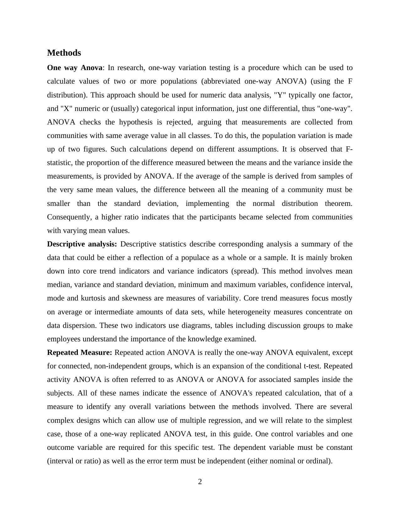
One way Anova: In research, one-way variation testing is a procedure which can be used to
calculate values of two or more populations (abbreviated one-way ANOVA) (using the F
distribution). This approach should be used for numeric data analysis, "Y" typically one factor,
and "X" numeric or (usually) categorical input information, just one differential, thus "one-way".
ANOVA checks the hypothesis is rejected, arguing that measurements are collected from
communities with same average value in all classes. To do this, the population variation is made
up of two figures. Such calculations depend on different assumptions. It is observed that F-
statistic, the proportion of the difference measured between the means and the variance inside the
measurements, is provided by ANOVA. If the average of the sample is derived from samples of
the very same mean values, the difference between all the meaning of a community must be
smaller than the standard deviation, implementing the normal distribution theorem.
Consequently, a higher ratio indicates that the participants became selected from communities
with varying mean values.
Descriptive analysis: Descriptive statistics describe corresponding analysis a summary of the
data that could be either a reflection of a populace as a whole or a sample. It is mainly broken
down into core trend indicators and variance indicators (spread). This method involves mean
median, variance and standard deviation, minimum and maximum variables, confidence interval,
mode and kurtosis and skewness are measures of variability. Core trend measures focus mostly
on average or intermediate amounts of data sets, while heterogeneity measures concentrate on
data dispersion. These two indicators use diagrams, tables including discussion groups to make
employees understand the importance of the knowledge examined.
Repeated Measure: Repeated action ANOVA is really the one-way ANOVA equivalent, except
for connected, non-independent groups, which is an expansion of the conditional t-test. Repeated
activity ANOVA is often referred to as ANOVA or ANOVA for associated samples inside the
subjects. All of these names indicate the essence of ANOVA's repeated calculation, that of a
measure to identify any overall variations between the methods involved. There are several
complex designs which can allow use of multiple regression, and we will relate to the simplest
case, those of a one-way replicated ANOVA test, in this guide. One control variables and one
outcome variable are required for this specific test. The dependent variable must be constant
(interval or ratio) as well as the error term must be independent (either nominal or ordinal).
2

Results
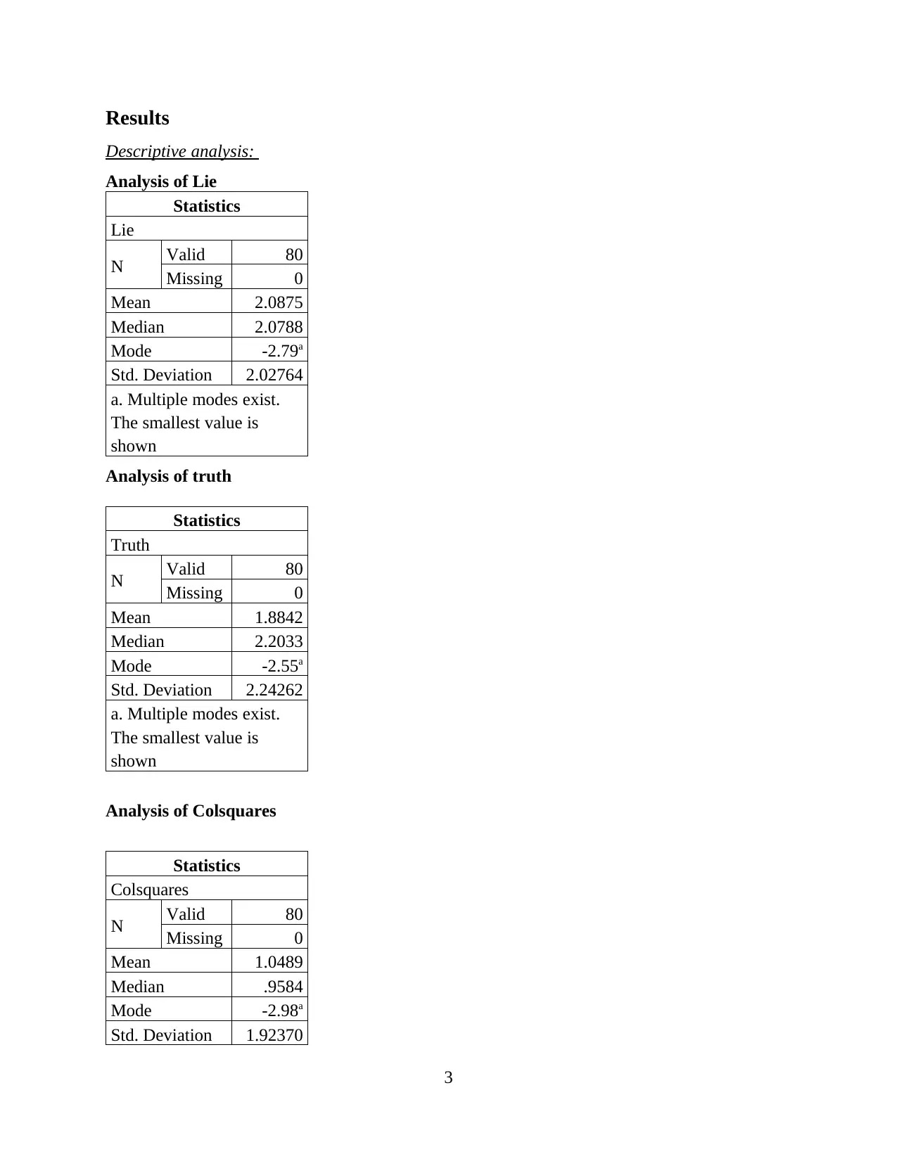
Descriptive analysis:
Analysis of Lie
Statistics
Lie
N Valid 80
Missing 0
Mean 2.0875
Median 2.0788
Mode -2.79a
Std. Deviation 2.02764
a. Multiple modes exist.
The smallest value is
shown
Analysis of truth
Statistics
Truth
N Valid 80
Missing 0
Mean 1.8842
Median 2.2033
Mode -2.55a
Std. Deviation 2.24262
a. Multiple modes exist.
The smallest value is
shown
Analysis of Colsquares
Statistics
Colsquares
N Valid 80
Missing 0
Mean 1.0489
Median .9584
Mode -2.98a
Std. Deviation 1.92370
3

a. Multiple modes exist.
The smallest value is
shown
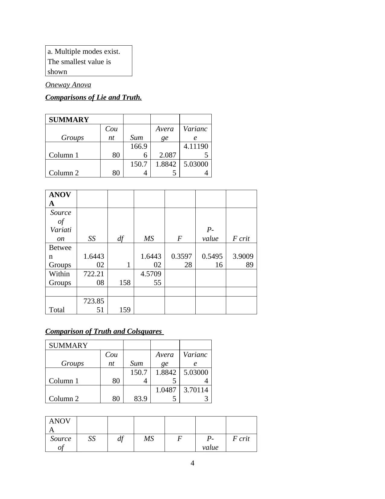
Oneway Anova
Comparisons of Lie and Truth.
SUMMARY
Groups
Cou
nt Sum
Avera
ge
Varianc
e
Column 1 80
166.9
6 2.087
4.11190
5
Column 2 80
150.7
4
1.8842
5
5.03000
4
ANOV
A
Source
of
Variati
on SS df MS F
P-
value F crit
Betwee
n
Groups
1.6443
02 1
1.6443
02
0.3597
28
0.5495
16
3.9009
89
Within
Groups
722.21
08 158
4.5709
55
Total
723.85
51 159
Comparison of Truth and Colsquares
SUMMARY
Groups
Cou
nt Sum
Avera
ge
Varianc
e
Column 1 80
150.7
4
1.8842
5
5.03000
4
Column 2 80 83.9
1.0487
5
3.70114
3
ANOV
A
Source
of
SS df MS F P-
value
F crit
4

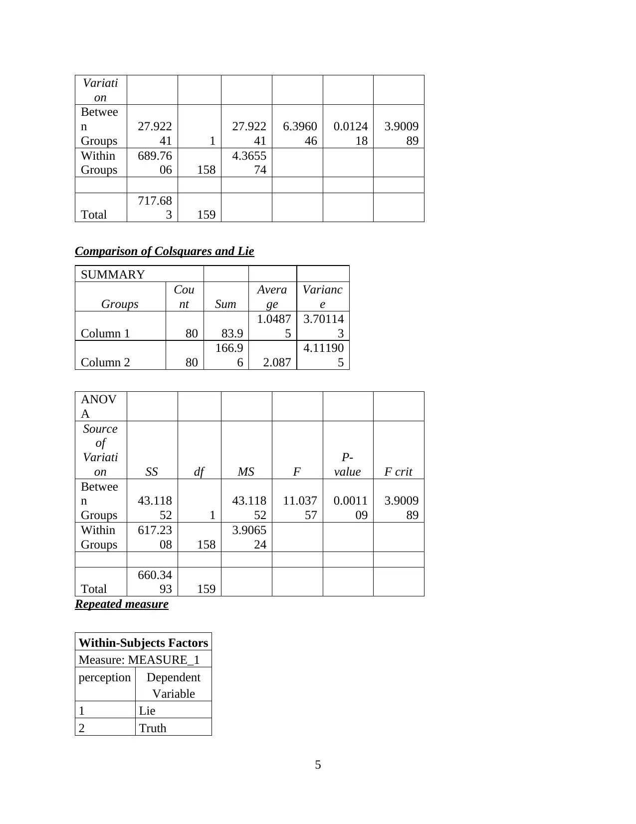
Variati
on
Betwee
n
Groups
27.922
41 1
27.922
41
6.3960
46
0.0124
18
3.9009
89
Within
Groups
689.76
06 158
4.3655
74
Total
717.68
3 159
Comparison of Colsquares and Lie
SUMMARY
Groups
Cou
nt Sum
Avera
ge
Varianc
e
Column 1 80 83.9
1.0487
5
3.70114
3
Column 2 80
166.9
6 2.087
4.11190
5
ANOV
A
Source
of
Variati
on SS df MS F
P-
value F crit
Betwee
n
Groups
43.118
52 1
43.118
52
11.037
57
0.0011
09
3.9009
89
Within
Groups
617.23
08 158
3.9065
24
Total
660.34
93 159
Repeated measure
Within-Subjects Factors
Measure: MEASURE_1
perception Dependent
Variable
1 Lie
2 Truth
5

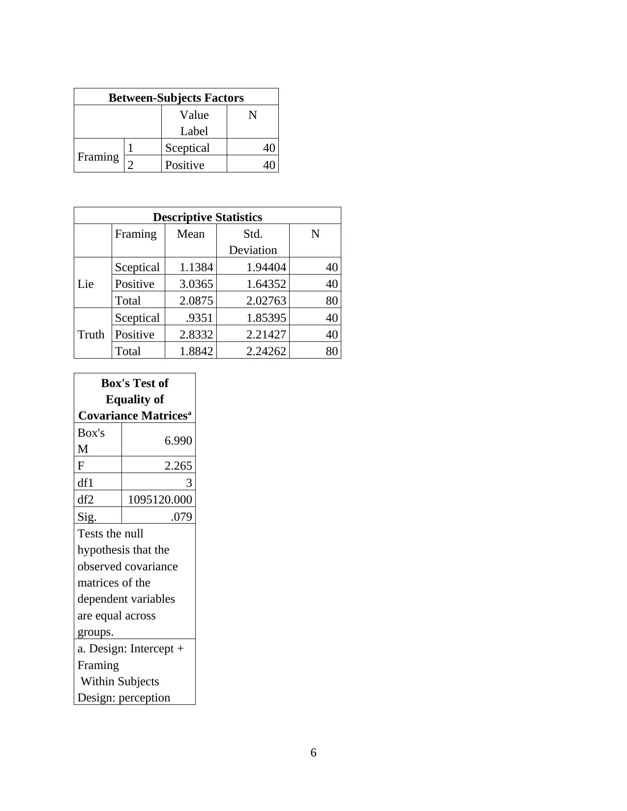
Between-Subjects Factors
Value
Label
N
Framing 1 Sceptical 40
2 Positive 40
Descriptive Statistics
Framing Mean Std.
Deviation
N
Lie
Sceptical 1.1384 1.94404 40
Positive 3.0365 1.64352 40
Total 2.0875 2.02763 80
Truth
Sceptical .9351 1.85395 40
Positive 2.8332 2.21427 40
Total 1.8842 2.24262 80
Box's Test of
Equality of
Covariance Matricesa
Box's
M 6.990
F 2.265
df1 3
df2 1095120.000
Sig. .079
Tests the null
hypothesis that the
observed covariance
matrices of the
dependent variables
are equal across
groups.
a. Design: Intercept +
Framing
Within Subjects
Design: perception
6

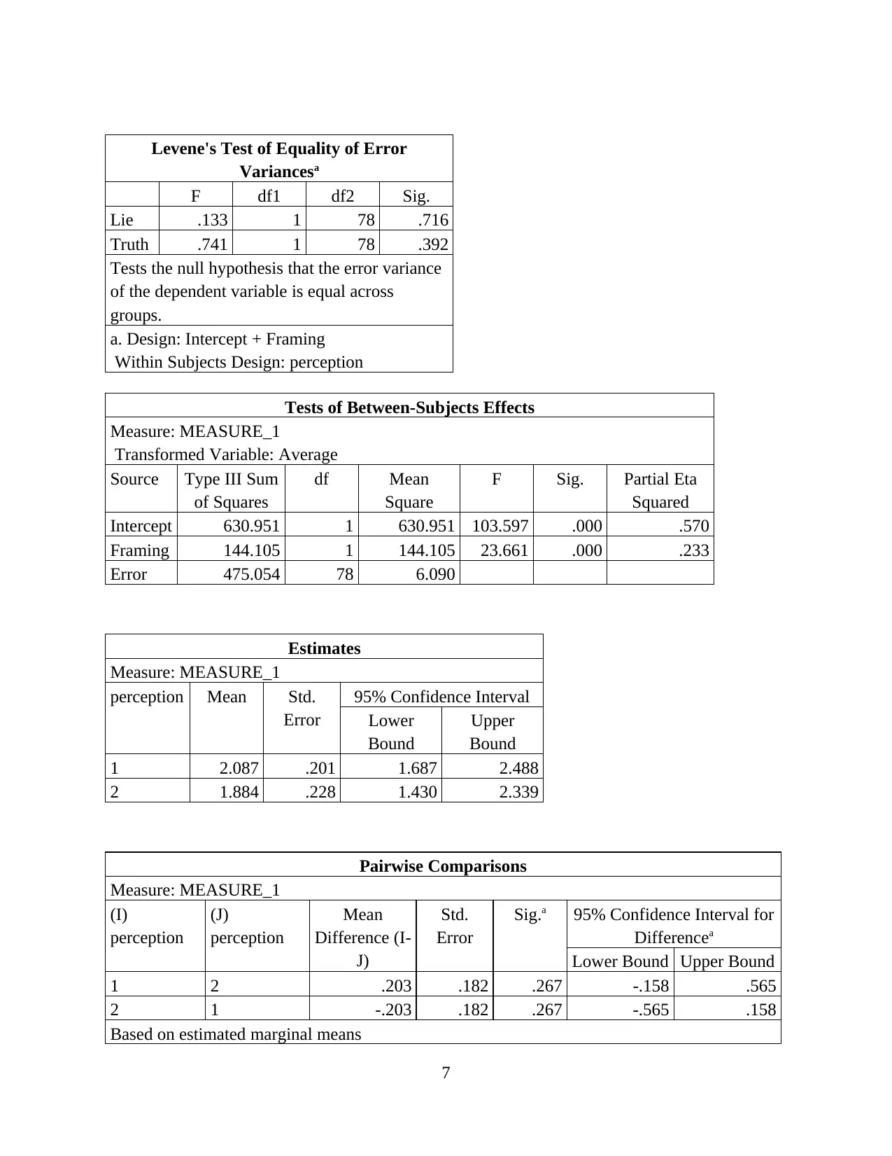
Levene's Test of Equality of Error
Variancesa
F df1 df2 Sig.
Lie .133 1 78 .716
Truth .741 1 78 .392
Tests the null hypothesis that the error variance
of the dependent variable is equal across
groups.
a. Design: Intercept + Framing
Within Subjects Design: perception
Tests of Between-Subjects Effects
Measure: MEASURE_1
Transformed Variable: Average
Source Type III Sum
of Squares
df Mean
Square
F Sig. Partial Eta
Squared
Intercept 630.951 1 630.951 103.597 .000 .570
Framing 144.105 1 144.105 23.661 .000 .233
Error 475.054 78 6.090
Estimates
Measure: MEASURE_1
perception Mean Std.
Error
95% Confidence Interval
Lower
Bound
Upper
Bound
1 2.087 .201 1.687 2.488
2 1.884 .228 1.430 2.339
Pairwise Comparisons
Measure: MEASURE_1
(I)
perception
(J)
perception
Mean
Difference (I-
J)
Std.
Error
Sig.a 95% Confidence Interval for
Differencea
Lower Bound Upper Bound
1 2 .203 .182 .267 -.158 .565
2 1 -.203 .182 .267 -.565 .158
Based on estimated marginal means
7

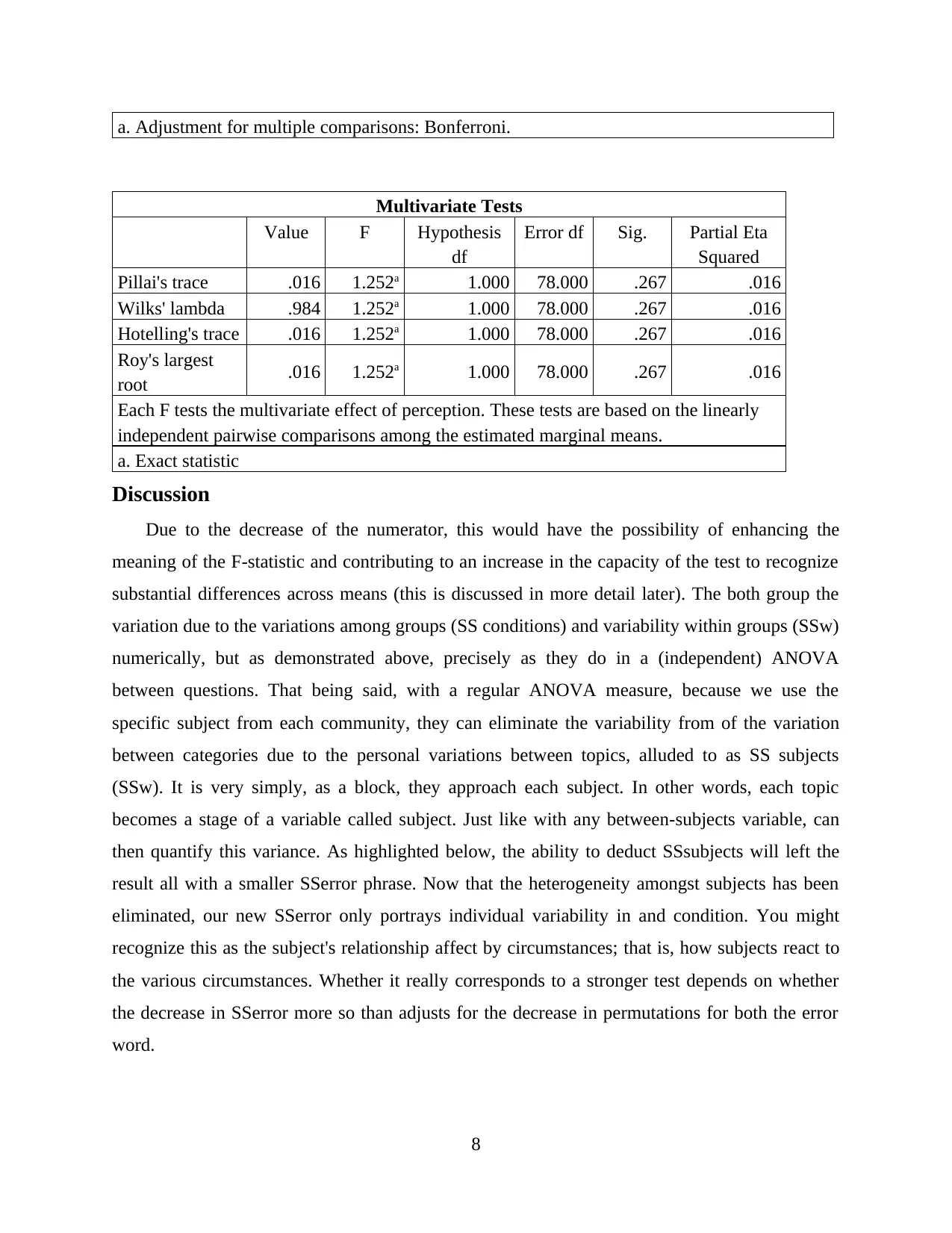
a. Adjustment for multiple comparisons: Bonferroni.
Multivariate Tests
Value F Hypothesis
df
Error df Sig. Partial Eta
Squared
Pillai's trace .016 1.252a 1.000 78.000 .267 .016
Wilks' lambda .984 1.252a 1.000 78.000 .267 .016
Hotelling's trace .016 1.252a 1.000 78.000 .267 .016
Roy's largest
root .016 1.252a 1.000 78.000 .267 .016
Each F tests the multivariate effect of perception. These tests are based on the linearly
independent pairwise comparisons among the estimated marginal means.
a. Exact statistic
Discussion
Due to the decrease of the numerator, this would have the possibility of enhancing the
meaning of the F-statistic and contributing to an increase in the capacity of the test to recognize
substantial differences across means (this is discussed in more detail later). The both group the
variation due to the variations among groups (SS conditions) and variability within groups (SSw)
numerically, but as demonstrated above, precisely as they do in a (independent) ANOVA
between questions. That being said, with a regular ANOVA measure, because we use the
specific subject from each community, they can eliminate the variability from of the variation
between categories due to the personal variations between topics, alluded to as SS subjects
(SSw). It is very simply, as a block, they approach each subject. In other words, each topic
becomes a stage of a variable called subject. Just like with any between-subjects variable, can
then quantify this variance. As highlighted below, the ability to deduct SSsubjects will left the
result all with a smaller SSerror phrase. Now that the heterogeneity amongst subjects has been
eliminated, our new SSerror only portrays individual variability in and condition. You might
recognize this as the subject's relationship affect by circumstances; that is, how subjects react to
the various circumstances. Whether it really corresponds to a stronger test depends on whether
the decrease in SSerror more so than adjusts for the decrease in permutations for both the error
word.
8

It is also discovered from the above, descriptive analysis that the mean value of lie for both
the group is 2.078, truth is 1.8 and colsquares is 1.04 approx which states that average mean is
for all the group is above the level of standard mean.
Conclusion
In the last of report, it is founded that quantitative analysis is the useful tool which involves
statistical calculation and equation which support in making the suitable results for the collected
variables including various categories. The reliable SPSS testing gives the detail compassion
between two factorial variables such as Lie and truth in order to define the perception of two
groups male and female. Thus it is also concluded that the ANOVA only fixes not tell the exact
values which means were different from one another. To regulate that, researchers would
essential to follow up with multiple comparisons (or post-hoc) tests.
9

REFERENCES
Books and Journals
Banerjee, M. and Mishra, M., 2017. Retail supply chain management practices in India: A
business intelligence perspective. Journal of Retailing and Consumer Services. 34.
pp.248-259.
Batra, D., 2018. Agile values or plan-driven aspects: Which factor contributes more toward the
success of data warehousing, business intelligence, and analytics project
development?. Journal of Systems and Software. 146. pp.249-262.
Vallurupalli, V. and Bose, I., 2018. Business intelligence for performance measurement: A case
based analysis. Decision Support Systems. 111. pp.72-85.
Villar, A and et. al., 2018. Integrating and analyzing medical and environmental data using ETL
and Business Intelligence tools. International journal of biometeorology. 62(6).
pp.1085-1095.
Zhou, C and et. al., 2020. A data-driven business intelligence system for large-scale semi-
automated logistics facilities. International Journal of Production Research. pp.1-19.
Zulfiqar, M and et. al., 2019, December. Use of Macro/Micro Models and Business Intelligence
tools for Energy Assessment and Scenario based Modeling. In 2019 4th International
Conference on Emerging Trends in Engineering, Sciences and Technology
(ICEEST) (pp. 1-7). IEEE.
10