Quantitative Analysis for Business

This article discusses the best methods for data collection, suitable sampling options, and correlation and regression analysis for take home pay and weekly food expenditure.

QUANTITATIVE ANALYSIS FOR BUSINESS
STUDENT NAME/ID
[Pick the date]

Part 1
(A) Online surveying or collecting data from email surveying is best possible method for the
researcher considering the underlying questions asked are factual and are less likely to be
misinterpreted. This method is also efficient in terms of cost and energy and money saving
which is vital considering that the samples need to be geographically distributed (Lieberman
et. al., 2015).
(B) Stratified random sampling is suitable option as it provides the sample which comprises the
attributes of the population in the same proportion in sample selected as the population
actually have. The conclusion based on the sample would be considered more reliable and
accurate if this sampling mechanism is adhered to (Hillier, 2016).
(C) The critical issues while collecting the data is to invite more people for the responses than
required so that accommodation can be done for responses not received along with
incomplete responses. Also, there can be potential delays in collection owing to late
responses. Also, since some individuals in the sample would not respond, hence the final
sample may be a little biased in terms of attribute distribution (Hair et. al., 2015).
Part 2
(A) For determining the suitable classes required, it is imperative that the data range ought to be
considered which highlights the values that ought to be represented. Also, the underlying
distribution must be considered using the dispersion indicators such as standard deviation.
Considering these, the optimum number of classes would be determined (Flick, 2015).
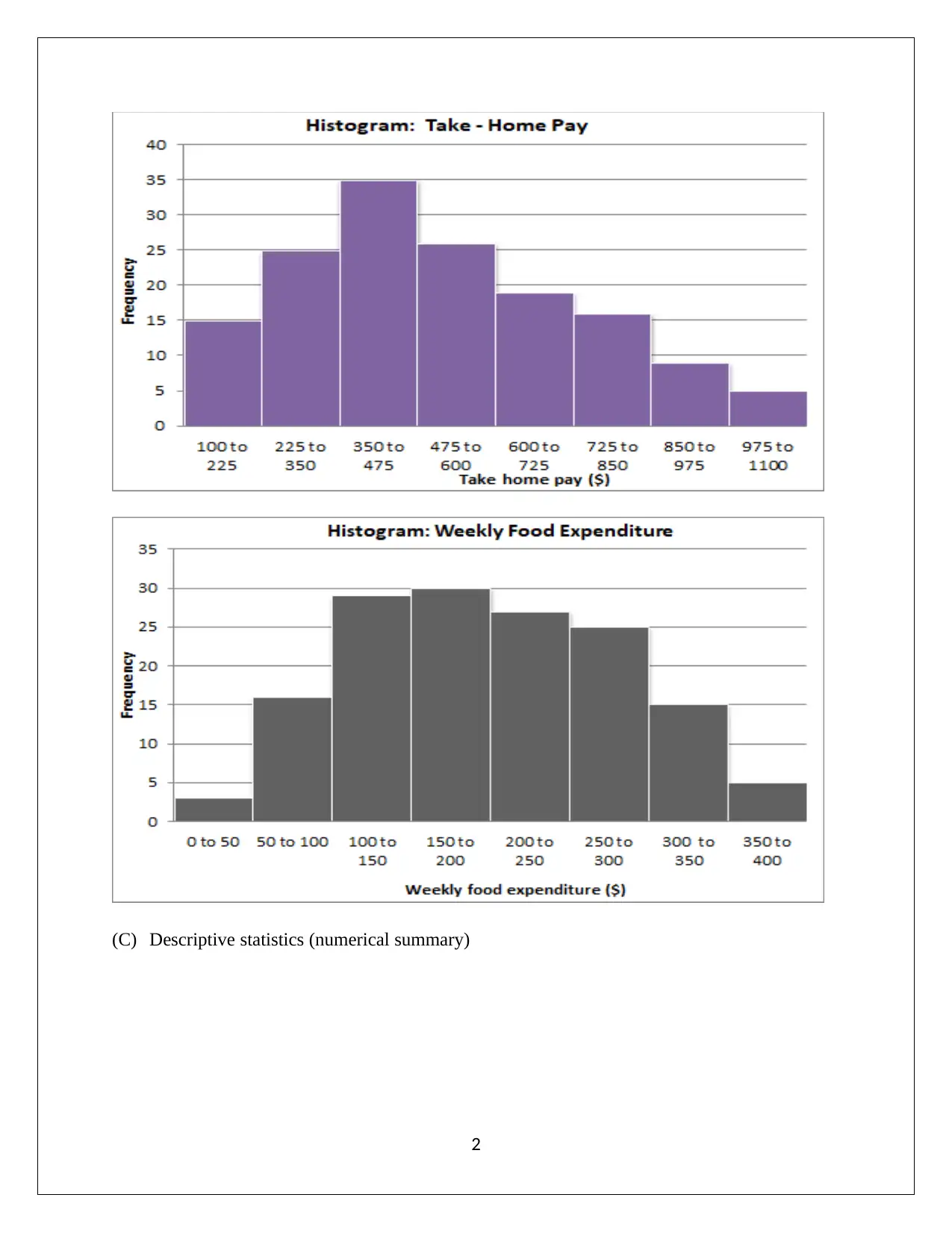
(B) Histogram
Take Home Pay
1

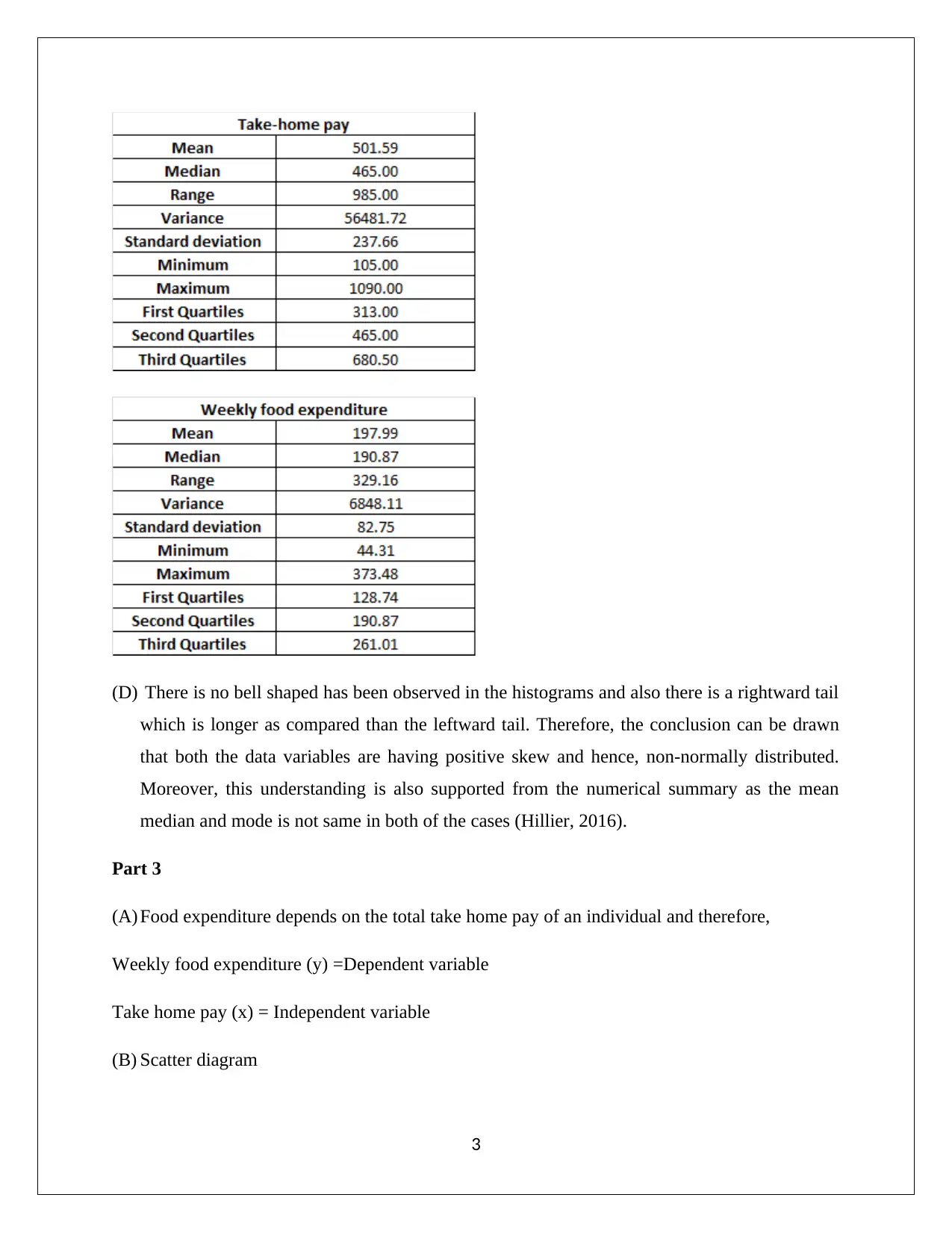
(C) Descriptive statistics (numerical summary)
2

(D) There is no bell shaped has been observed in the histograms and also there is a rightward tail
which is longer as compared than the leftward tail. Therefore, the conclusion can be drawn
that both the data variables are having positive skew and hence, non-normally distributed.
Moreover, this understanding is also supported from the numerical summary as the mean
median and mode is not same in both of the cases (Hillier, 2016).
Part 3
(A) Food expenditure depends on the total take home pay of an individual and therefore,
Weekly food expenditure (y) =Dependent variable
Take home pay (x) = Independent variable
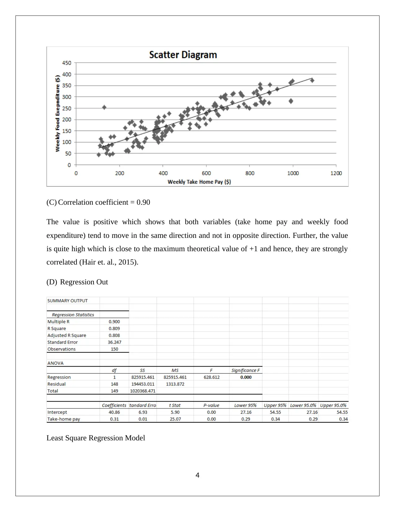
(B) Scatter diagram
3

(C) Correlation coefficient = 0.90
The value is positive which shows that both variables (take home pay and weekly food
expenditure) tend to move in the same direction and not in opposite direction. Further, the value
is quite high which is close to the maximum theoretical value of +1 and hence, they are strongly
correlated (Hair et. al., 2015).
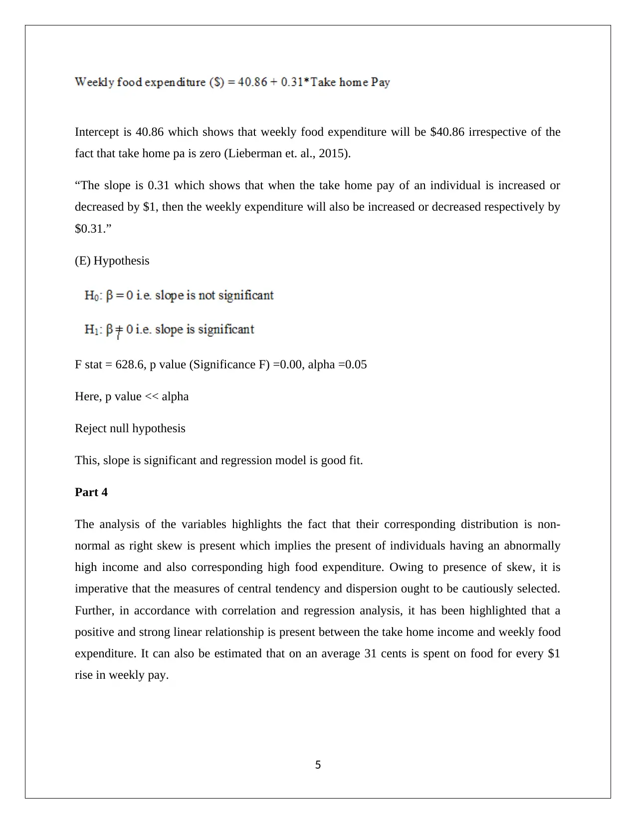
(D) Regression Out
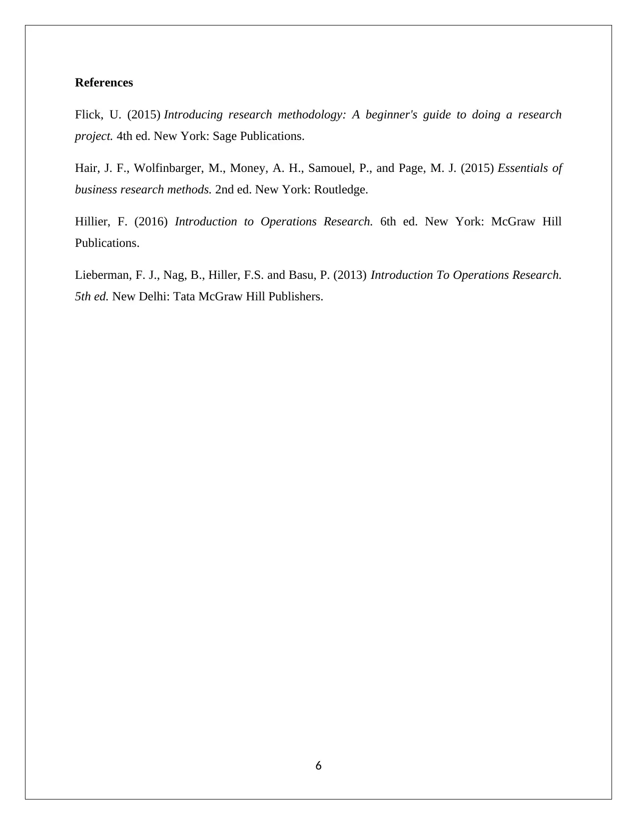
Least Square Regression Model
4

Intercept is 40.86 which shows that weekly food expenditure will be $40.86 irrespective of the
fact that take home pa is zero (Lieberman et. al., 2015).
“The slope is 0.31 which shows that when the take home pay of an individual is increased or
decreased by $1, then the weekly expenditure will also be increased or decreased respectively by
$0.31.”
(E) Hypothesis
F stat = 628.6, p value (Significance F) =0.00, alpha =0.05
Here, p value << alpha
Reject null hypothesis
This, slope is significant and regression model is good fit.
Part 4
The analysis of the variables highlights the fact that their corresponding distribution is non-
normal as right skew is present which implies the present of individuals having an abnormally
high income and also corresponding high food expenditure. Owing to presence of skew, it is
imperative that the measures of central tendency and dispersion ought to be cautiously selected.
Further, in accordance with correlation and regression analysis, it has been highlighted that a
positive and strong linear relationship is present between the take home income and weekly food
expenditure. It can also be estimated that on an average 31 cents is spent on food for every $1
rise in weekly pay.
5

References
Flick, U. (2015) Introducing research methodology: A beginner's guide to doing a research
project. 4th ed. New York: Sage Publications.
Hair, J. F., Wolfinbarger, M., Money, A. H., Samouel, P., and Page, M. J. (2015) Essentials of
business research methods. 2nd ed. New York: Routledge.
Hillier, F. (2016) Introduction to Operations Research. 6th ed. New York: McGraw Hill
Publications.
Lieberman, F. J., Nag, B., Hiller, F.S. and Basu, P. (2013) Introduction To Operations Research.
5th ed. New Delhi: Tata McGraw Hill Publishers.
6