Quantitative Analysis for Business - Take Home Pay and Weekly Food Expenditure

This study focuses on the effect of take home pay on weekly food expenditure. The researcher conducted a cross sectional survey to establish the linear association between the variables of the study. The scatter plot and regression analysis showed a high positive correlation between take home pay and weekly food expenditure in Australia.

~ 1 ~
Quantitative Analysis for Business
Course Code: QAB105
Semester: 2
Year: 2018

~ 2 ~
Answer Part 1
(a) The sample data was collected for two fields, take home pay and weekly food
expenditure. The effect of take home pay on weekly food expenditure would have been
the field of research. Hence, cross-sectional survey would have been the choice for the
researcher with properly designed questionnaire, to facilitate a cause and effect study.
(b) The collected sample was observed to be targeted towards salaried people, where the
distribution pattern of the histogram was inclined more towards mid level income group.
Hence, convenience sampling would have been the choice for the survey (Norman, &
Streiner, 2008).
(c) Due to convenience sampling, the sample might be biased in nature. The probability of
excluding various data points (salaried people) could have generated a bias sample during
the data collection procedure.
Answer Part 2
(a) The researcher might have used the rule where k is the least number and denotes the
number of intervals and n is the number of observations. Here, the least value of k = 8 that
satisfied the inequality where n = 150. The choice of eight intervals ensured that the
histograms reflected exact nature of the distributions, especially regarding the skewness and
kurtosis of the variables (Scott, 2009).
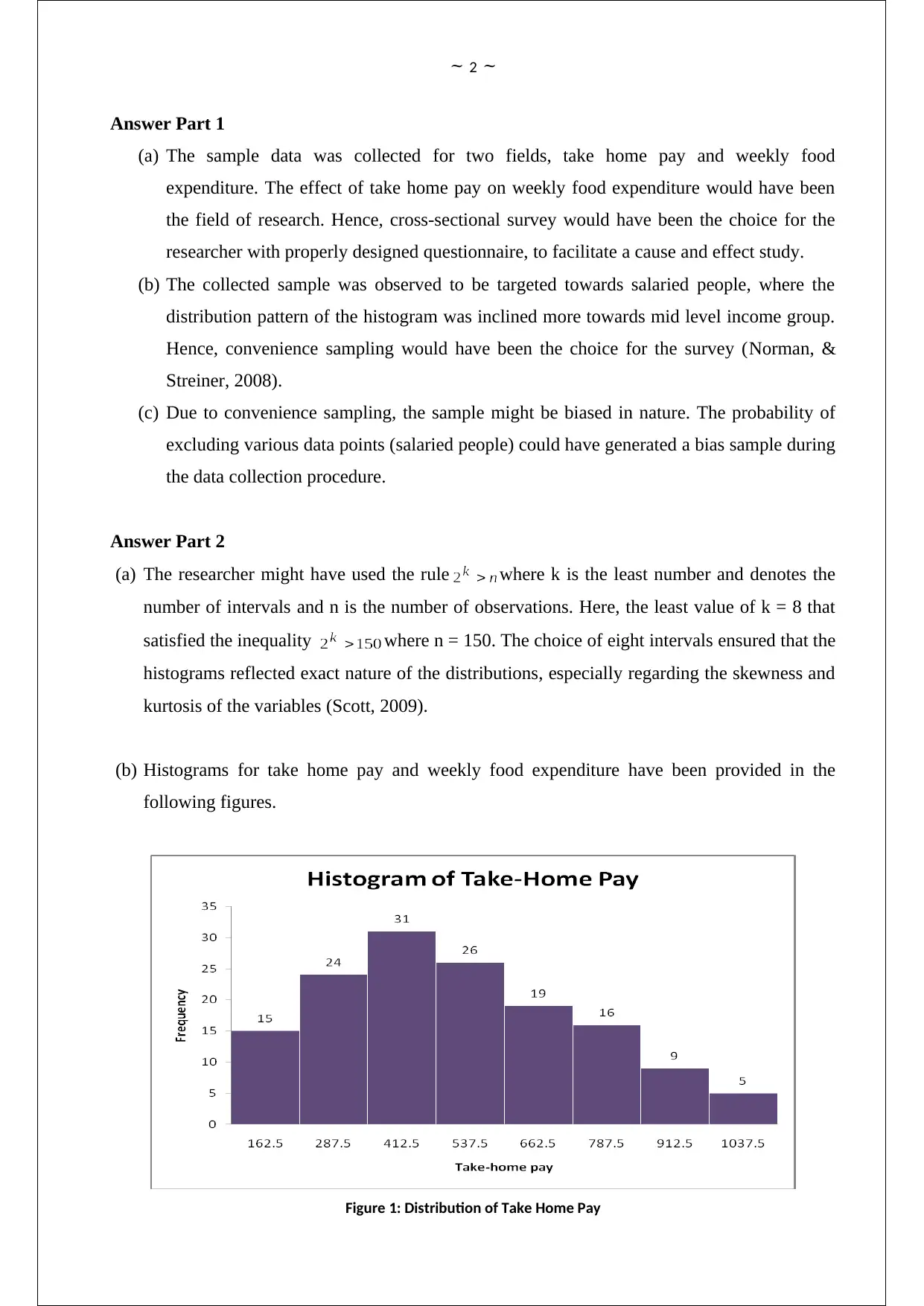
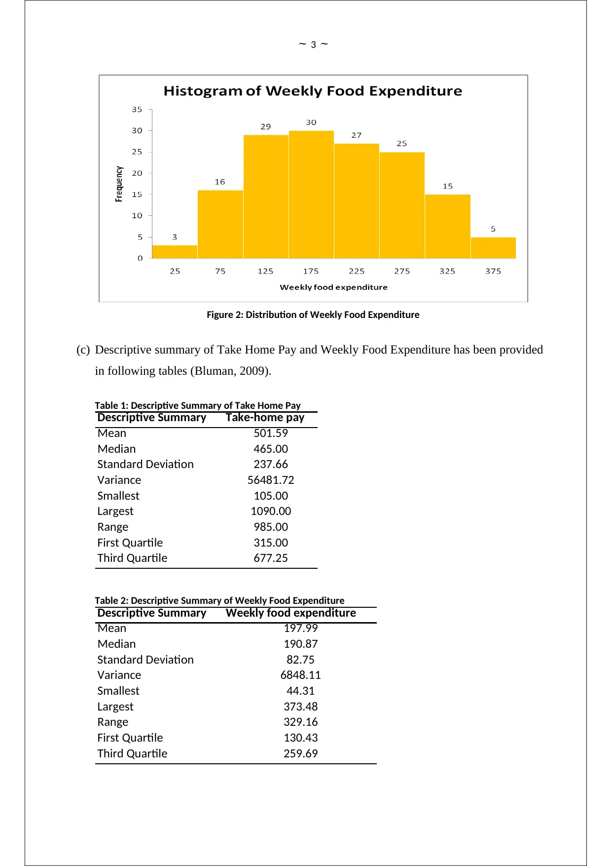
(b) Histograms for take home pay and weekly food expenditure have been provided in the
following figures.
Figure 1: Distribution of Take Home Pay

~ 3 ~
Figure 2: Distribution of Weekly Food Expenditure
(c) Descriptive summary of Take Home Pay and Weekly Food Expenditure has been provided
in following tables (Bluman, 2009).
Table 1: Descriptive Summary of Take Home Pay
Descriptive Summary Take-home pay
Mean 501.59
Median 465.00
Standard Deviation 237.66
Variance 56481.72
Smallest 105.00
Largest 1090.00
Range 985.00
First Quartile 315.00
Third Quartile 677.25
Table 2: Descriptive Summary of Weekly Food Expenditure
Descriptive Summary Weekly food expenditure
Mean 197.99
Median 190.87
Standard Deviation 82.75
Variance 6848.11
Smallest 44.31
Largest 373.48
Range 329.16
First Quartile 130.43
Third Quartile 259.69

~ 4 ~
(d) The mean and median of the distribution of take home pay were 501.59 and 465. The
median was less than the mean of the distribution, signifying that the distribution was right
skewed. It was observed that the trend of the histogram was also positively skewed,
establishing the estimation from the descriptive values.
The mean and median of the distribution of take home pay were 197.99 and 190.87. The
median was somewhat less than the mean of the distribution, signifying that the distribution
was a little right skewed. It was observed that the trend of the histogram was almost normal,
establishing the estimation from the descriptive values.
Answer Part 3
(a) The most probable and likely choice of independent variable was take home pay, and the
inclination for dependent variable was towards weekly food expenditure.
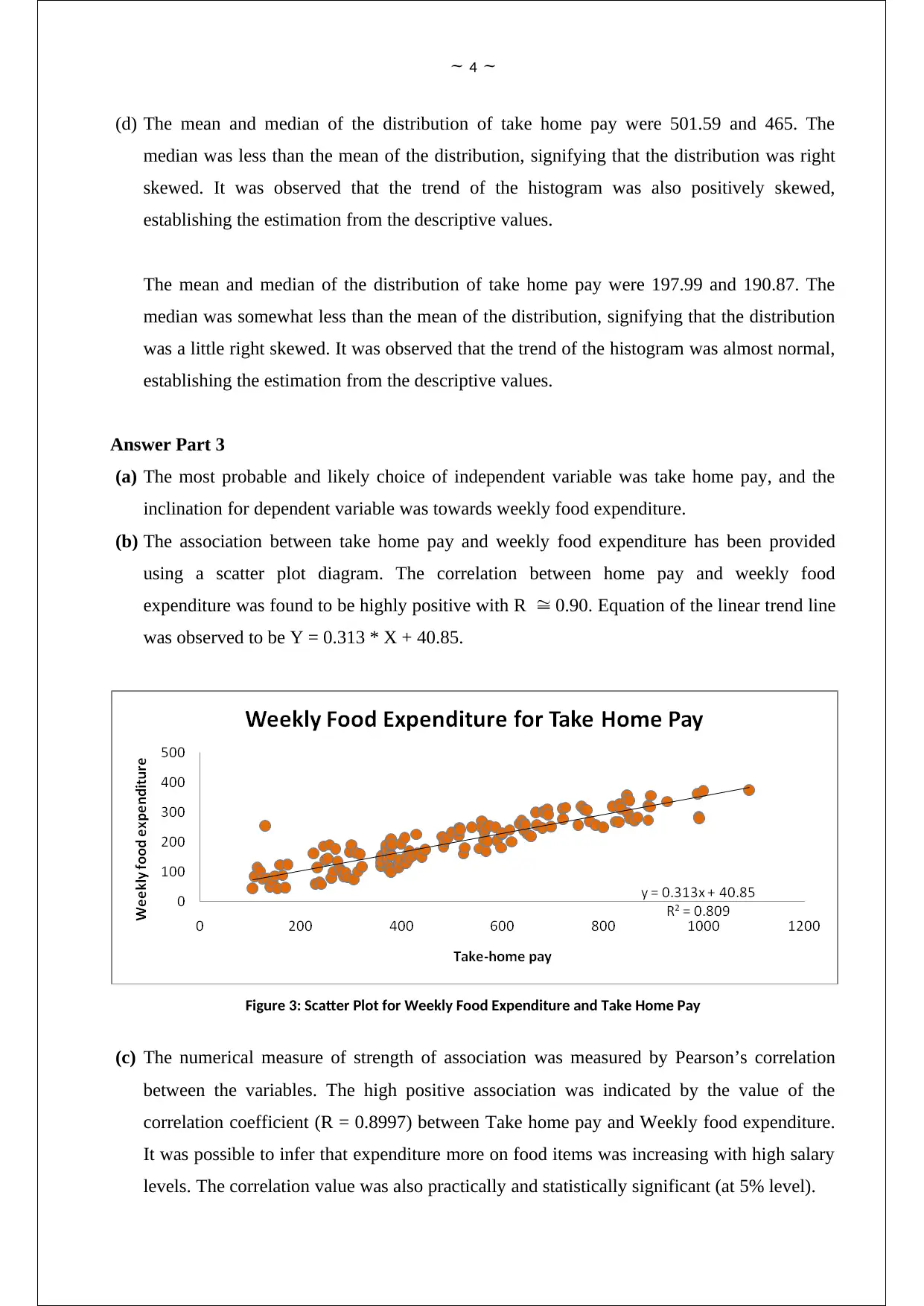
(b) The association between take home pay and weekly food expenditure has been provided
using a scatter plot diagram. The correlation between home pay and weekly food
expenditure was found to be highly positive with R 0.90. Equation of the linear trend line
was observed to be Y = 0.313 * X + 40.85.
Figure 3: Scatter Plot for Weekly Food Expenditure and Take Home Pay
(c) The numerical measure of strength of association was measured by Pearson’s correlation
between the variables. The high positive association was indicated by the value of the
correlation coefficient (R = 0.8997) between Take home pay and Weekly food expenditure.
It was possible to infer that expenditure more on food items was increasing with high salary
levels. The correlation value was also practically and statistically significant (at 5% level).

~ 5 ~
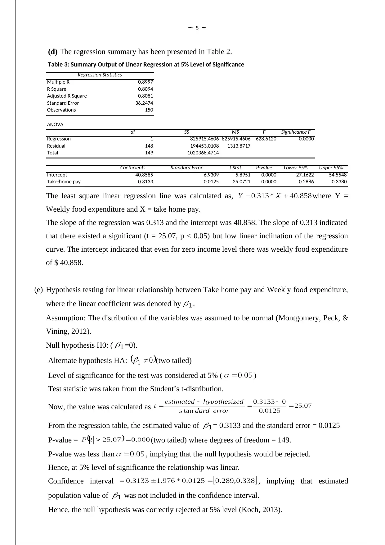
(d) The regression summary has been presented in Table 2.
Table 3: Summary Output of Linear Regression at 5% Level of Significance
Regression Statistics
Multiple R 0.8997
R Square 0.8094
Adjusted R Square 0.8081
Standard Error 36.2474
Observations 150
ANOVA
df SS MS F Significance F
Regression 1 825915.4606 825915.4606 628.6120 0.0000
Residual 148 194453.0108 1313.8717
Total 149 1020368.4714
Coefficients Standard Error t Stat P-value Lower 95% Upper 95%
Intercept 40.8585 6.9309 5.8951 0.0000 27.1622 54.5548
Take-home pay 0.3133 0.0125 25.0721 0.0000 0.2886 0.3380
The least square linear regression line was calculated as, where Y =
Weekly food expenditure and X = take home pay.
The slope of the regression was 0.313 and the intercept was 40.858. The slope of 0.313 indicated
that there existed a significant (t = 25.07, p < 0.05) but low linear inclination of the regression
curve. The intercept indicated that even for zero income level there was weekly food expenditure
of $ 40.858.
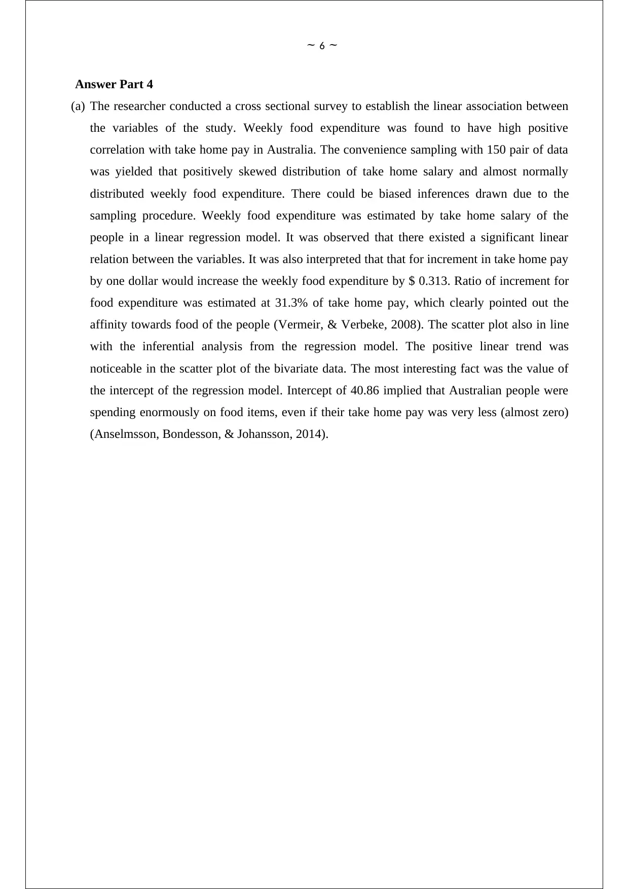
(e) Hypothesis testing for linear relationship between Take home pay and Weekly food expenditure,
where the linear coefficient was denoted by .
Assumption: The distribution of the variables was assumed to be normal (Montgomery, Peck, &
Vining, 2012).
Null hypothesis H0: ( =0).
Alternate hypothesis HA: (two tailed)
Level of significance for the test was considered at 5% ( )
Test statistic was taken from the Student’s t-distribution.
Now, the value was calculated as
From the regression table, the estimated value of = 0.3133 and the standard error = 0.0125
P-value = (two tailed) where degrees of freedom = 149.
P-value was less than , implying that the null hypothesis would be rejected.
Hence, at 5% level of significance the relationship was linear.
Confidence interval = , implying that estimated
population value of was not included in the confidence interval.
Hence, the null hypothesis was correctly rejected at 5% level (Koch, 2013).

~ 6 ~
Answer Part 4
(a) The researcher conducted a cross sectional survey to establish the linear association between
the variables of the study. Weekly food expenditure was found to have high positive
correlation with take home pay in Australia. The convenience sampling with 150 pair of data
was yielded that positively skewed distribution of take home salary and almost normally
distributed weekly food expenditure. There could be biased inferences drawn due to the
sampling procedure. Weekly food expenditure was estimated by take home salary of the
people in a linear regression model. It was observed that there existed a significant linear
relation between the variables. It was also interpreted that that for increment in take home pay
by one dollar would increase the weekly food expenditure by $ 0.313. Ratio of increment for
food expenditure was estimated at 31.3% of take home pay, which clearly pointed out the
affinity towards food of the people (Vermeir, & Verbeke, 2008). The scatter plot also in line
with the inferential analysis from the regression model. The positive linear trend was
noticeable in the scatter plot of the bivariate data. The most interesting fact was the value of
the intercept of the regression model. Intercept of 40.86 implied that Australian people were
spending enormously on food items, even if their take home pay was very less (almost zero)
(Anselmsson, Bondesson, & Johansson, 2014).

~ 7 ~
References
Anselmsson, J., Vestman Bondesson, N., & Johansson, U. (2014). Brand image and customers'
willingness to pay a price premium for food brands. Journal of Product & Brand
Management, 23(2), 90-102.
Bluman, A. G. (2009). Elementary statistics: A step by step approach. New York: McGraw-Hill
Higher Education.
Koch, K. R. (2013). Parameter estimation and hypothesis testing in linear models. Springer
Science & Business Media.
Montgomery, D. C., Peck, E. A., & Vining, G. G. (2012). Introduction to linear regression
analysis (Vol. 821). John Wiley & Sons.
Norman, G. R., & Streiner, D. L. (2008). Biostatistics: the bare essentials. PMPH-USA.
Scott, D. W. (2009). Sturges' rule. Wiley Interdisciplinary Reviews: Computational Statistics,
1(3), 303-306.
Vermeir, I., & Verbeke, W. (2008). Sustainable food consumption among young adults in
Belgium: Theory of planned behaviour and the role of confidence and values. Ecological
economics, 64(3), 542-553.