Quantitative Analysis of the Business 2022

Running Header: Quantitative Analysis of Business 1
Quantitative Analysis for Business
Student’s name:
Student’s ID:
Institution:

Quantitative Analysis of Business 2
Part 1
(a)
The survey method that the research could use is an online survey. The method is suitable due to the
popularity of technology and the ease of designing and deploying the surveys (Roberts & Allen,
2015). Consequently, the respondents are given ample space and time to respond to the answers
thereby given unbiased responses.
(b)
The best method for selecting the sample is through the use of random sampling. Random sampling
involves selecting a representative group from the population being studied (Emerson, 2015). Using
random sampling is the best suited since it represents the target population and eliminates sampling
bias.
(c)
When collecting data through random sampling, the researcher may face challenges since it requires
a lot of time and effort and it is very expensive in carrying out (Etikan & Bala, 2017).
Part 2
(a)
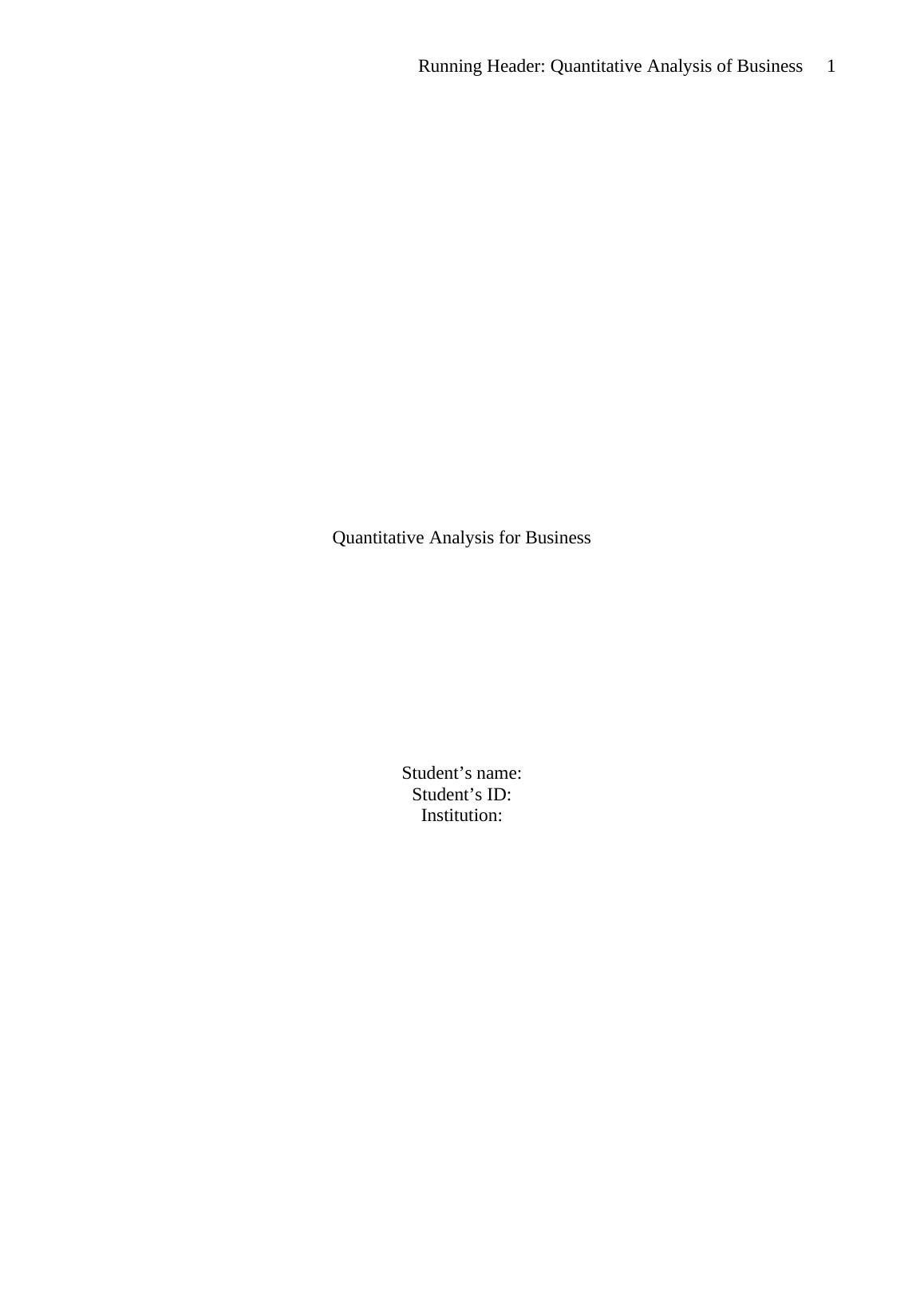
There is no rule with regard to the number of classes that one should use (Frankfort-Nachmias &
Leon-Guerrero, 2017). The decision to use 10 as the number of classes is attributed to the nature of
the data set. The data set used is relatively large and the aim of using a histogram is to have
meaningful information. Hence, using a class of 10 is the most appropriate in coming up with
information that is useful and can be used in data analysis.
(b)
Figure 1: Television Hours Histogram

Quantitative Analysis of Business 3
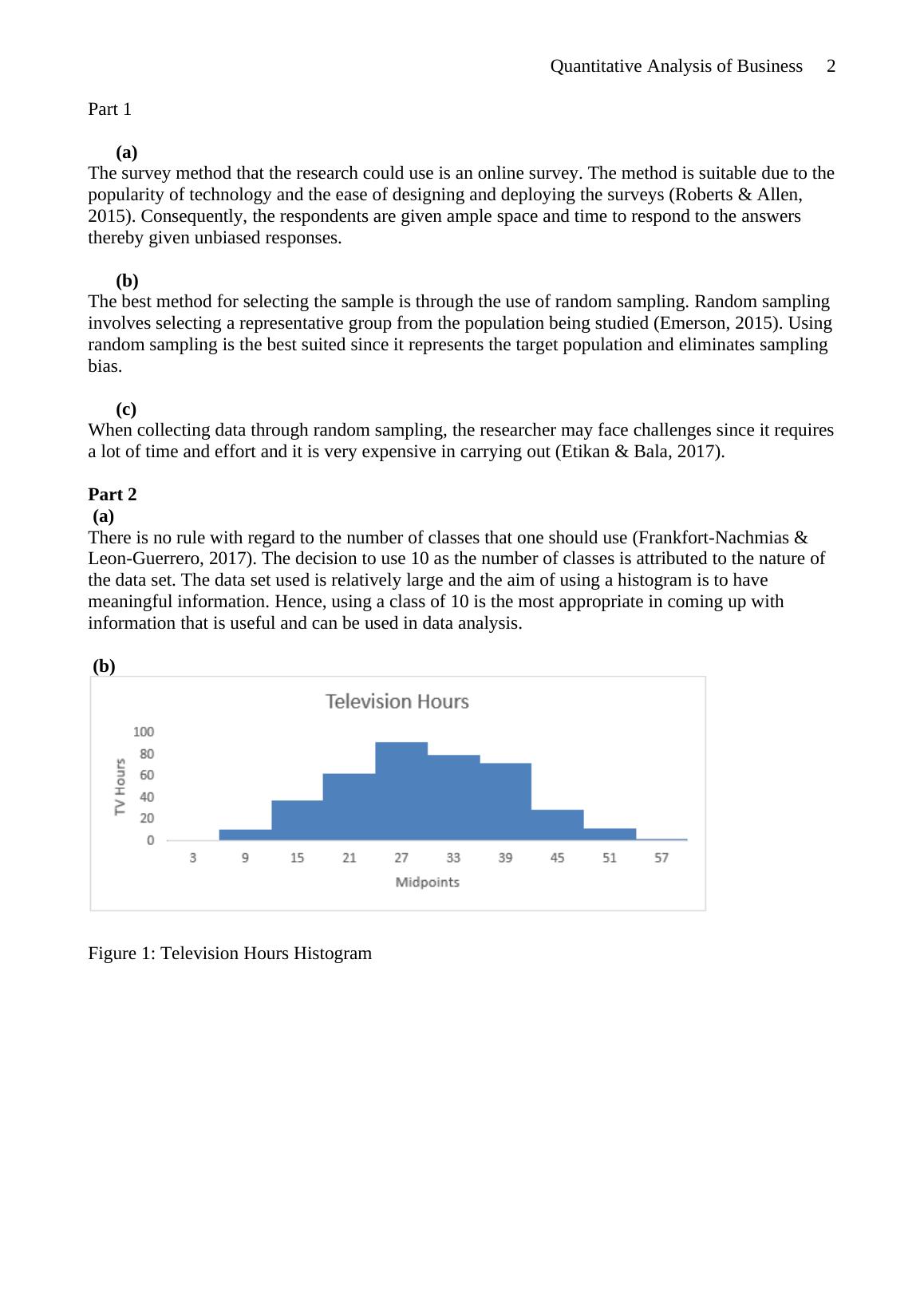
Figure 2: Total Debt Histogram
(c)
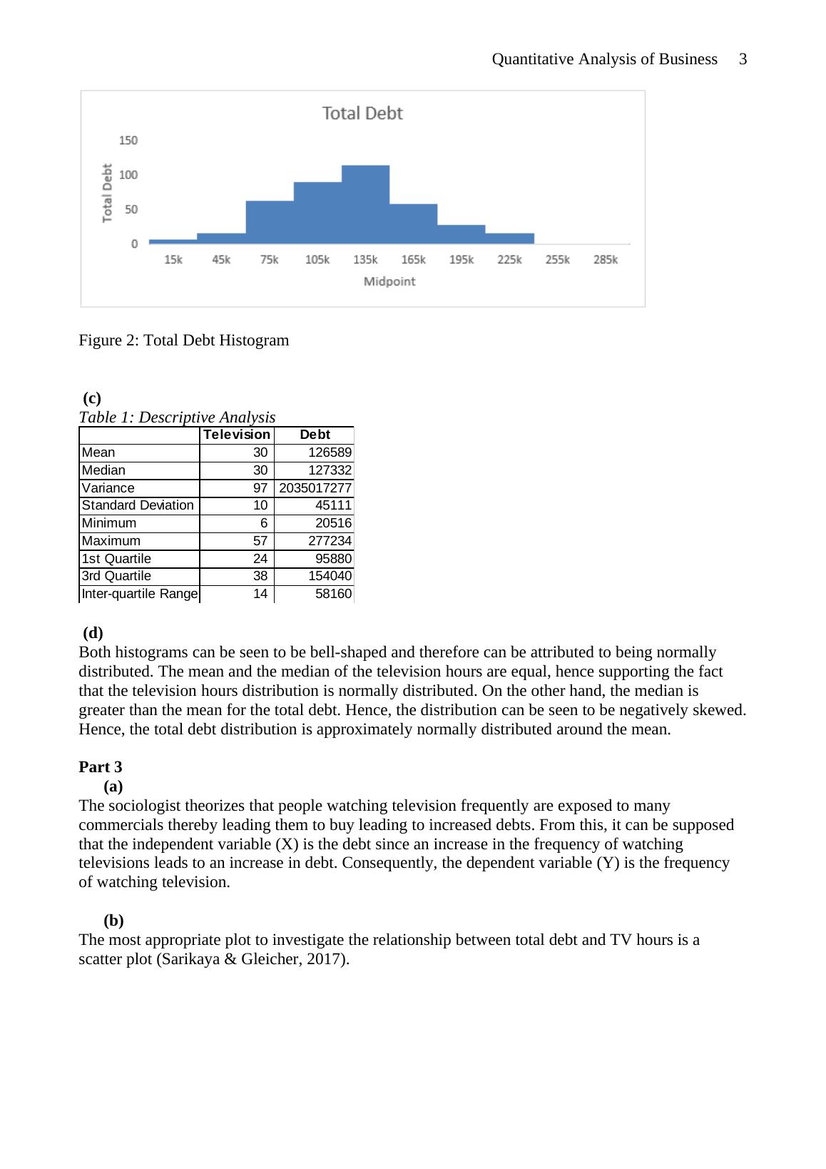
Table 1: Descriptive Analysis
Television Debt
Mean 30 126589
Median 30 127332
Variance 97 2035017277
Standard Deviation 10 45111
Minimum 6 20516
Maximum 57 277234
1st Quartile 24 95880
3rd Quartile 38 154040
Inter-quartile Range 14 58160
(d)
Both histograms can be seen to be bell-shaped and therefore can be attributed to being normally
distributed. The mean and the median of the television hours are equal, hence supporting the fact
that the television hours distribution is normally distributed. On the other hand, the median is
greater than the mean for the total debt. Hence, the distribution can be seen to be negatively skewed.
Hence, the total debt distribution is approximately normally distributed around the mean.
Part 3
(a)
The sociologist theorizes that people watching television frequently are exposed to many
commercials thereby leading them to buy leading to increased debts. From this, it can be supposed
that the independent variable (X) is the debt since an increase in the frequency of watching
televisions leads to an increase in debt. Consequently, the dependent variable (Y) is the frequency
of watching television.
(b)
The most appropriate plot to investigate the relationship between total debt and TV hours is a
scatter plot (Sarikaya & Gleicher, 2017).