UGB 108: Quantitative Methods for Business Report Analysis
VerifiedAdded on 2023/01/11
|12
|2635
|69
Report
AI Summary
This report presents solutions to a quantitative methods for business assignment, addressing key concepts and techniques. It begins with an introduction to quantitative methods and their role in decision-making. Question 1 focuses on descriptive statistics, including the calculation of mean and standard deviation for access time data, along with an analysis of sampling methods and cumulative frequency distributions. Question 2 delves into regression analysis, calculating regression coefficients and making a business decision based on these coefficients. Finally, Question 4 explores correlation, calculating Spearman’s rank correlation coefficient and Pearson’s product moment correlation. The report concludes with an overview of the findings and includes a comprehensive reference list.
Quantitative Methods for
Business
Business
Paraphrase This Document
Need a fresh take? Get an instant paraphrase of this document with our AI Paraphraser
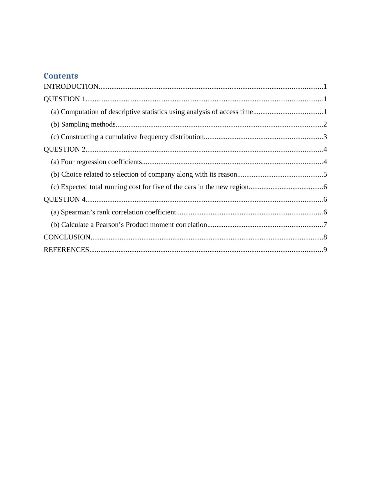
Contents
INTRODUCTION...........................................................................................................................1
QUESTION 1..................................................................................................................................1
(a) Computation of descriptive statistics using analysis of access time......................................1
(b) Sampling methods..................................................................................................................2
(c) Constructing a cumulative frequency distribution.................................................................3
QUESTION 2..................................................................................................................................4
(a) Four regression coefficients...................................................................................................4
(b) Choice related to selection of company along with its reason...............................................5
(c) Expected total running cost for five of the cars in the new region.........................................6
QUESTION 4..................................................................................................................................6
(a) Spearman’s rank correlation coefficient................................................................................6
(b) Calculate a Pearson’s Product moment correlation...............................................................7
CONCLUSION................................................................................................................................8
REFERENCES................................................................................................................................9

⊘ This is a preview!⊘
Do you want full access?
Subscribe today to unlock all pages.

Trusted by 1+ million students worldwide
INTRODUCTION
Quantitative Methods for Business are the techniques which are used by an organisation to
collect and analyse their data in such a way that can assist in the procedure of decision making.
There are various quantitative methods which are based on statistical and mathematical measures
(Kumar and Belwal, 2017). The main aim of this report is to develop an understanding about the
role of quantitative methods and how they can be used in real life practices.
In this present report, three questions will be solved which are based on mathematical and
statistical concepts. These questions are related to descriptive statistical tools mean and standard
deviation, regression and correlation.
QUESTION 1
(a) Computation of descriptive statistics using analysis of access time
I. Determination of mean access time
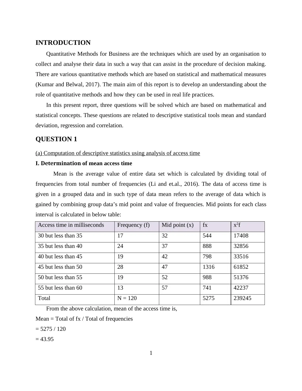
Mean is the average value of entire data set which is calculated by dividing total of
frequencies from total number of frequencies (Li and et.al., 2016). The data of access time is
given in a grouped data and in such type of data mean refers to the average of data which is
gained by combining group data’s mid point and value of frequencies. Mid points for each class
interval is calculated in below table:
Access time in milliseconds Frequency (f) Mid point (x) fx x2f
30 but less than 35 17 32 544 17408
35 but less than 40 24 37 888 32856
40 but less than 45 19 42 798 33516
45 but less than 50 28 47 1316 61852
50 but less than 55 19 52 988 51376
55 but less than 60 13 57 741 42237
Total N = 120 5275 239245
From the above calculation, mean of the access time is,
Mean = Total of fx / Total of frequencies
= 5275 / 120
= 43.95
1
Paraphrase This Document
Need a fresh take? Get an instant paraphrase of this document with our AI Paraphraser
II. Determination of standard deviation of the access time
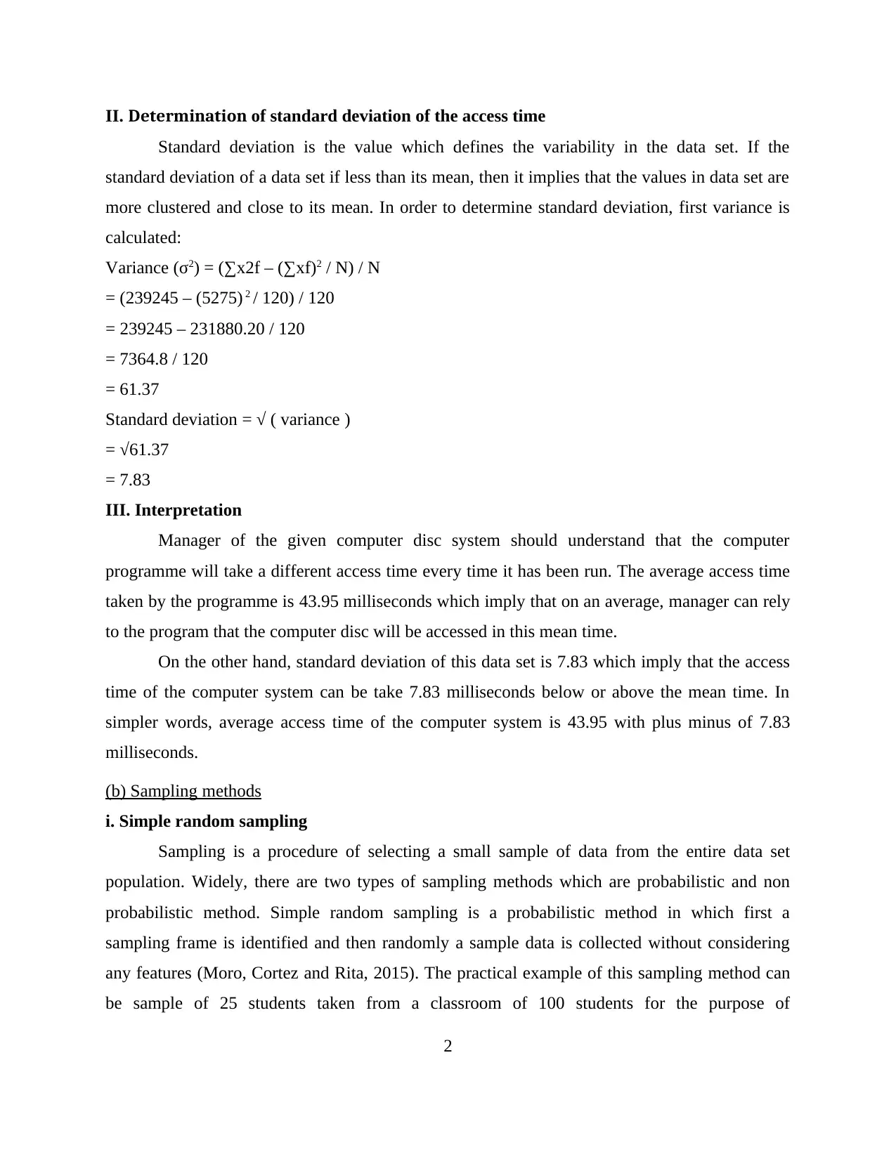
Standard deviation is the value which defines the variability in the data set. If the
standard deviation of a data set if less than its mean, then it implies that the values in data set are
more clustered and close to its mean. In order to determine standard deviation, first variance is
calculated:
Variance (σ2) = (∑x2f – (∑xf)2 / N) / N
= (239245 – (5275) 2 / 120) / 120
= 239245 – 231880.20 / 120
= 7364.8 / 120
= 61.37
Standard deviation = √ ( variance )
= √61.37
= 7.83
III. Interpretation
Manager of the given computer disc system should understand that the computer
programme will take a different access time every time it has been run. The average access time
taken by the programme is 43.95 milliseconds which imply that on an average, manager can rely
to the program that the computer disc will be accessed in this mean time.
On the other hand, standard deviation of this data set is 7.83 which imply that the access
time of the computer system can be take 7.83 milliseconds below or above the mean time. In
simpler words, average access time of the computer system is 43.95 with plus minus of 7.83
milliseconds.
(b) Sampling methods
i. Simple random sampling
Sampling is a procedure of selecting a small sample of data from the entire data set
population. Widely, there are two types of sampling methods which are probabilistic and non
probabilistic method. Simple random sampling is a probabilistic method in which first a
sampling frame is identified and then randomly a sample data is collected without considering
any features (Moro, Cortez and Rita, 2015). The practical example of this sampling method can
be sample of 25 students taken from a classroom of 100 students for the purpose of
2
photographing them for annual bulletin. In this each student in the classroom of 100 students has
equal chance to be selected.
ii. Quota sampling
This type of sampling is non probabilistic in which entire population is divided into
various groups which are called quotas and then a sample of equal individuals are selected from
each quota which can represent their respective quota (Rittman, 2012). This type of sampling is
opposite from simple random sampling and requires skills and capabilities. Practical example of
this method can be the blood samples taken from five individuals from each residential area of
United Kingdom to check the impact of the diseases like Malaria.
iv. Cluster sampling
This sampling method is similar to quota sampling as in both of the methods entire
population is divided into groups. But unlike quota sampling, in cluster sampling, entire
population is divided into some groups according to some features and traits. Each group is
referred as clusters and a sample from each cluster is taken. This technique is much complex
than the other two defined above which raises the chances of error as well. The practical example
of this clustering can be the sample of two students taken from each of the age group in order to
analyse their body mass.
v. Systematic sampling
This is also a type of probabilistic sampling in which an interval is selected randomly
which is known as interval point. Once, the interval point is selected then samples from the entire
data set are gathered at that interval point which is required to be fixed (Muley and Joshi, 2015).
A practical example of this method can be the selection of every 5th student in the class to test
their body mass. This method of sampling is a biased method in which every individual does not
have the equal chance to be selected.
(c) Constructing a cumulative frequency distribution
Cumulative frequency distribution is a representation of class intervals and their
frequencies so that total values of frequencies after each interval can be gained (Renso,
Spaccapietra and Zimányi, 2013). A distribution table for a dataset is developed below:
S.No. Class interval
Frequency
(f)
Cumulative
frequency (cf)
Cumulative
relative frequency
Cumulative
percentage
3
⊘ This is a preview!⊘
Do you want full access?
Subscribe today to unlock all pages.

Trusted by 1+ million students worldwide
frequency
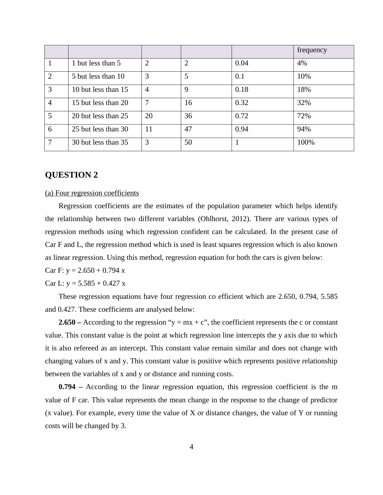
1 1 but less than 5 2 2 0.04 4%
2 5 but less than 10 3 5 0.1 10%
3 10 but less than 15 4 9 0.18 18%
4 15 but less than 20 7 16 0.32 32%
5 20 but less than 25 20 36 0.72 72%
6 25 but less than 30 11 47 0.94 94%
7 30 but less than 35 3 50 1 100%
QUESTION 2
(a) Four regression coefficients
Regression coefficients are the estimates of the population parameter which helps identify
the relationship between two different variables (Ohlhorst, 2012). There are various types of
regression methods using which regression confident can be calculated. In the present case of
Car F and L, the regression method which is used is least squares regression which is also known
as linear regression. Using this method, regression equation for both the cars is given below:
Car F: y = 2.650 + 0.794 x
Car L: y = 5.585 + 0.427 x
These regression equations have four regression co efficient which are 2.650, 0.794, 5.585
and 0.427. These coefficients are analysed below:
2.650 – According to the regression “y = mx + c”, the coefficient represents the c or constant
value. This constant value is the point at which regression line intercepts the y axis due to which
it is also refereed as an intercept. This constant value remain similar and does not change with
changing values of x and y. This constant value is positive which represents positive relationship
between the variables of x and y or distance and running costs.
0.794 – According to the linear regression equation, this regression coefficient is the m
value of F car. This value represents the mean change in the response to the change of predictor
(x value). For example, every time the value of X or distance changes, the value of Y or running
costs will be changed by 3.
4
Paraphrase This Document
Need a fresh take? Get an instant paraphrase of this document with our AI Paraphraser
5.585 – Similar to 2.650, this value is the constant variable for L car which remains constant
for the entire dataset. This value is the point at which regression line has crossed the Y axis.
0.427 – This value is the m value for L car which implies that with every changing distance
of L car, its running cost will also change by 0.427.
(b) Choice related to selection of company along with its reason
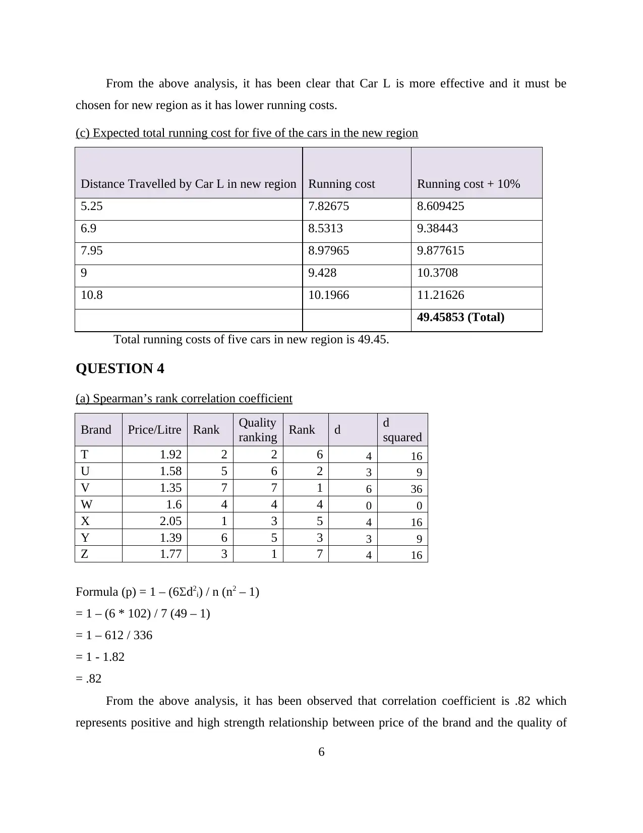
The distances travelled by Car F and L are increased by 50% and are recorded in table below:
Using the data above, it can be seen that Mean value of distance travelled for Car F and
for Car L is 12. Using the regression equation mean running costs for both the cars is calculated
as follows:
Car F: y = 2.650 + 0.794 * 12.00
y = 12.178
Mean running cost of Car F is 12.178
Car L: y = 5.585 + 0.427 * 12.00
y = 10.709
Mean running costs of Car L is 10.709.
5
From the above analysis, it has been clear that Car L is more effective and it must be
chosen for new region as it has lower running costs.
(c) Expected total running cost for five of the cars in the new region
Distance Travelled by Car L in new region Running cost Running cost + 10%
5.25 7.82675 8.609425
6.9 8.5313 9.38443
7.95 8.97965 9.877615
9 9.428 10.3708
10.8 10.1966 11.21626
49.45853 (Total)
Total running costs of five cars in new region is 49.45.
QUESTION 4
(a) Spearman’s rank correlation coefficient
Brand Price/Litre Rank Quality
ranking Rank d d
squared
T 1.92 2 2 6 4 16
U 1.58 5 6 2 3 9
V 1.35 7 7 1 6 36
W 1.6 4 4 4 0 0
X 2.05 1 3 5 4 16
Y 1.39 6 5 3 3 9
Z 1.77 3 1 7 4 16
Formula (p) = 1 – (6Σd2i) / n (n2 – 1)
= 1 – (6 * 102) / 7 (49 – 1)
= 1 – 612 / 336
= 1 - 1.82
= .82
From the above analysis, it has been observed that correlation coefficient is .82 which
represents positive and high strength relationship between price of the brand and the quality of
6
⊘ This is a preview!⊘
Do you want full access?
Subscribe today to unlock all pages.

Trusted by 1+ million students worldwide
the brand (Russom, 2011), due to which it can be said that consumer generally gets value for
their money.
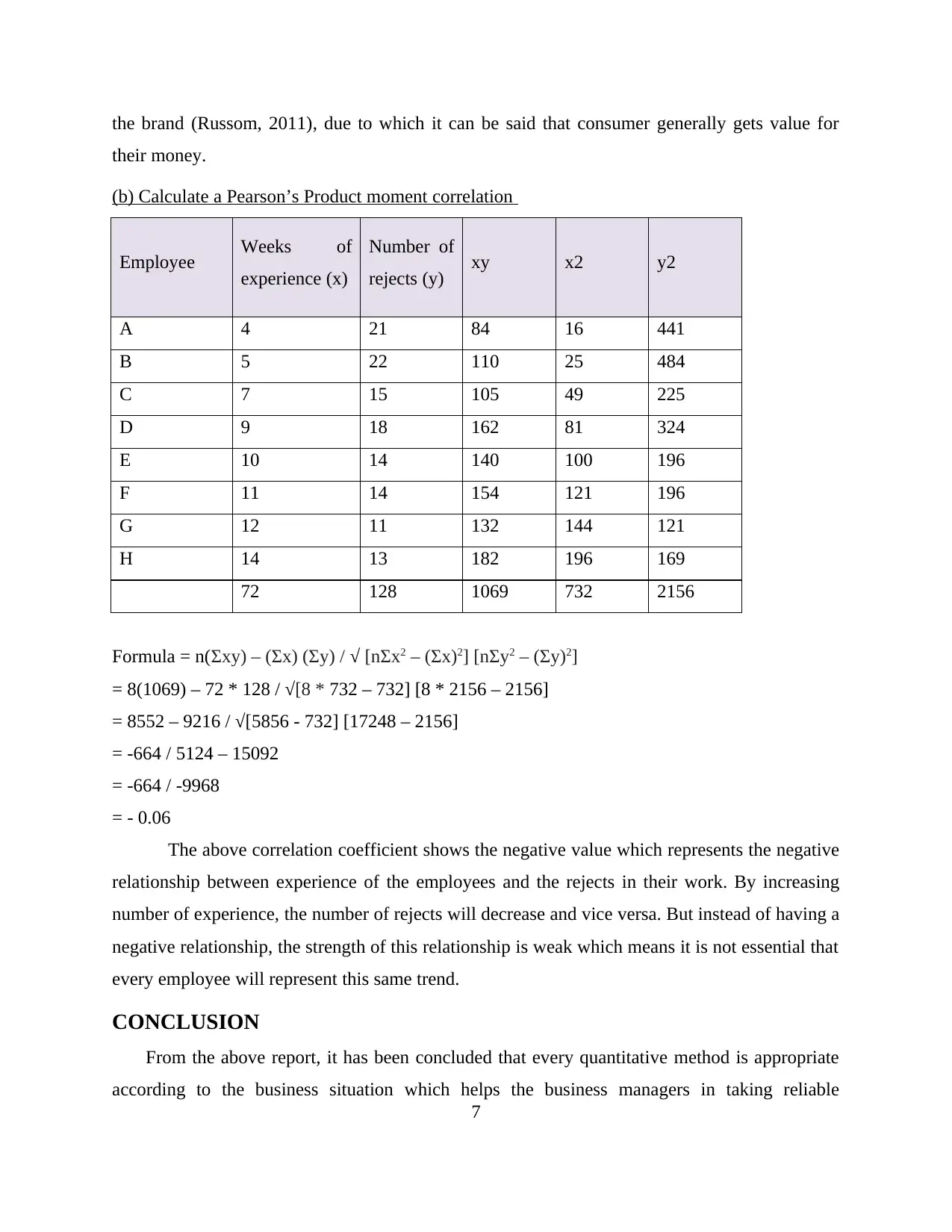
(b) Calculate a Pearson’s Product moment correlation
Employee Weeks of
experience (x)
Number of
rejects (y) xy x2 y2
A 4 21 84 16 441
B 5 22 110 25 484
C 7 15 105 49 225
D 9 18 162 81 324
E 10 14 140 100 196
F 11 14 154 121 196
G 12 11 132 144 121
H 14 13 182 196 169
72 128 1069 732 2156
Formula = n(Σxy) – (Σx) (Σy) / √ [nΣx2 – (Σx)2] [nΣy2 – (Σy)2]
= 8(1069) – 72 * 128 / √[8 * 732 – 732] [8 * 2156 – 2156]
= 8552 – 9216 / √[5856 - 732] [17248 – 2156]
= -664 / 5124 – 15092
= -664 / -9968
= - 0.06
The above correlation coefficient shows the negative value which represents the negative
relationship between experience of the employees and the rejects in their work. By increasing
number of experience, the number of rejects will decrease and vice versa. But instead of having a
negative relationship, the strength of this relationship is weak which means it is not essential that
every employee will represent this same trend.
CONCLUSION
From the above report, it has been concluded that every quantitative method is appropriate
according to the business situation which helps the business managers in taking reliable
7
Paraphrase This Document
Need a fresh take? Get an instant paraphrase of this document with our AI Paraphraser
decisions which further helps in growth and survival of the business. The above report is
summarised to few methods which are used in business and these methods were regression,
correlation and descriptive statistics. It also has been found that correlation and regression co
efficient helps in determining the relationship between two variables. These methods can also
provide the nature and strength of that relationship. By analysing few sampling methods, a
conclusion has been gained that sample random sampling and cluster sampling methods are
highly used in real life practices by investigators.
8
REFERENCES
Books and Journals
Kumar, S.M. and Belwal, M., 2017, August. Performance dashboard: Cutting-edge business
intelligence and data visualization. In 2017 International Conference On Smart
Technologies For Smart Nation (SmartTechCon) (pp. 1201-1207). IEEE.
Li, S. and et.al., 2016. Geospatial big data handling theory and methods: A review and research
challenges. ISPRS journal of Photogrammetry and Remote Sensing. 115. pp.119-133.
Moro, S., Cortez, P. and Rita, P., 2015. Business intelligence in banking: A literature analysis
from 2002 to 2013 using text mining and latent Dirichlet allocation. Expert Systems with
Applications. 42(3). pp.1314-1324.
Muley, P. and Joshi, A., 2015. Application of data mining techniques for customer segmentation
in real time business intelligence. International Journal of Innovative Research in
Advanced Engineering. 2(4). pp.106-109.
Ohlhorst, F.J., 2012. Big data analytics: turning big data into big money (Vol. 65). John Wiley
& Sons.
Renso, C., Spaccapietra, S. and Zimányi, E. eds., 2013. Mobility Data. Cambridge University
Press.
Rittman, M., 2012. Oracle Business Intelligence 11g Developers Guide. McGraw-Hill Osborne
Media.
Russom, P., 2011. Big data analytics. TDWI best practices report, fourth quarter, 19(4), pp.1-34.
9
⊘ This is a preview!⊘
Do you want full access?
Subscribe today to unlock all pages.

Trusted by 1+ million students worldwide
1 out of 12
Related Documents
Your All-in-One AI-Powered Toolkit for Academic Success.
+13062052269
info@desklib.com
Available 24*7 on WhatsApp / Email
![[object Object]](/_next/static/media/star-bottom.7253800d.svg)
Unlock your academic potential
Copyright © 2020–2026 A2Z Services. All Rights Reserved. Developed and managed by ZUCOL.


