QAB105 Quantitative Analysis for Business: A Detailed Report, 2018

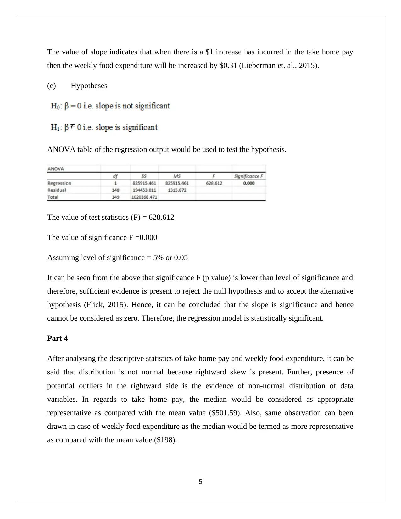
This report presents a quantitative analysis of business data, focusing on the relationship between take-home pay and weekly food expenditure. The analysis employs stratified random sampling and addresses potential data collection issues. Descriptive statistics, including histograms and numerical summaries, reveal a positive skew in the data. Regression analysis indicates a strong positive correlation between the variables, with a correlation coefficient of 0.90. The regression equation (y = 40.86 + 0.31x) suggests that for every $1 increase in take-home pay, weekly food expenditure increases by $0.31. Hypothesis testing confirms the statistical significance of the regression model. The report concludes that the variables are strongly correlated, validating the understanding that food expenditure is a function of income. Desklib offers a variety of similar solved assignments and past papers for students.

QUANTITATIVE ANALYSIS FOR BUSINESS
STUDENT NAME/ID
[Pick the date]

Part 1
(a) The researcher may use online survey as the nature of the research questions is factual
and does not require approaching the target population face to face. Also, collecting the
data through online surveying is quite easy and also leads to cost and time saving.
Further, sample can easily be collected from large population such as across the country
without much hassle (Flick, 2015).
(b) Stratified random sampling method is considered as appropriate sampling method to
draw the sample from the population. The main reason behind selecting this method is
that the extracted sample would be a true representation of the population. Further, the
sample obtained from this sampling would comprise of all the requisite attributes in the
same proportion as the population. Also, the statistically techniques apply on this sample
would provide more accurate result (Lieberman et. al., 2015).
(c) There are some key issues that may arise while collecting the data for the analysis. It is
possible that some of the individuals in the sample may not respond or provide
incomplete data. Thus, the researcher may have to approach many peoples as compared
with the decided sample size and hence, would be an issue (Hillier, 2016).
Part 2
(a) Maximum and minimum value of the given data set is the key parameters to decide the
class interval for the frequency distribution. The different between the maximum and
minimum value would be divided by the required number of classes which provides a
defined class interval for the analysis (Hair et. al., 2015).
(b) Histogram
Variable 1: Take Home Pay
1

Variable 2: Weekly food expenditure
(c) Numerical summary of the variables
2

(d) It can be seen from the above shown histograms that there is a long right ward tail which
is the indicative of the existence of positive skew in the data sets. Further, in both of the
above cases the mean value has exceeded the median value. It is evident of the fact that
rightward skew is present in the data for both the variables (Flick, 2015).
Part 3
(a) The variable ‘take home pay’ would be considered as independent variable whereas
variable ‘weekly food expenditure’ would be considered as dependent variable. The
reason behind this understanding is that the weekly food expenditure depends on the
weekly take home pay of the person (Hair et. al., 2015).
(b) The appropriate plot to represent the association between the variable is scatter plot.
3

(c) The correlation coefficient between take home pay and weekly food expenditure is
computed and comes out to be 0.90. It can be seen that the value is positive which
implies that correlation between take home pay and weekly food expenditure will move
in same direction only. Further, the positive association represents that as the take home
pay increases then the weekly food expenditure will also increase. It is apparent that the
value of correlation coefficient (0.90) is close to +1 which indicates that strength of
correlation between the variables is strong (Hillier, 2016).
(d) Regression output
Regression Equation
y=40.86+0.31 x
Weekly food expenditure( $)=40.86+(0.31∗Take home pay )
Interpretation:
 Intercept: 40.86
The value of intercept indicates that when the take home pay is 0 then the weekly food
expenditure will be $40.86.
 Slope: 0.31
4

The value of slope indicates that when there is a $1 increase has incurred in the take home pay
then the weekly food expenditure will be increased by $0.31 (Lieberman et. al., 2015).
(e) Hypotheses
ANOVA table of the regression output would be used to test the hypothesis.
The value of test statistics (F) = 628.612
The value of significance F =0.000
Assuming level of significance = 5% or 0.05
It can be seen from the above that significance F (p value) is lower than level of significance and
therefore, sufficient evidence is present to reject the null hypothesis and to accept the alternative
hypothesis (Flick, 2015). Hence, it can be concluded that the slope is significance and hence
cannot be considered as zero. Therefore, the regression model is statistically significant.
Part 4
After analysing the descriptive statistics of take home pay and weekly food expenditure, it can be
said that distribution is not normal because rightward skew is present. Further, presence of
potential outliers in the rightward side is the evidence of non-normal distribution of data
variables. In regards to take home pay, the median would be considered as appropriate
representative as compared with the mean value ($501.59). Also, same observation can been
drawn in case of weekly food expenditure as the median would be termed as more representative
as compared with the mean value ($198).
5

It can be said based on the above discussion, that variables take home pay and weekly food
expenditure are strongly correlated. This has been derived from high correlation coefficient and
regression analysis. It is quite obvious that food expenditure is a function of income and thus, the
conclusion has been validated in the study. Further, it is apparent from the above analysis that
when the take home pay is increased by $1 then the total weekly food expenditure will also
increase by $0.31.
6

References
Flick, U. (2015) Introducing research methodology: A beginner's guide to doing a research
project. 4th ed. New York: Sage Publications.
Hair, J. F., Wolfinbarger, M., Money, A. H., Samouel, P., and Page, M. J. (2015) Essentials of
business research methods. 2nd ed. New York: Routledge.
Hillier, F. (2016) Introduction to Operations Research. 6th ed. New York: McGraw Hill
Publications.
Lieberman, F. J., Nag, B., Hiller, F.S. and Basu, P. (2013) Introduction To Operations Research.
5th ed. New Delhi: Tata McGraw Hill Publishers.
7