Comprehensive Report: Quantitative Analysis of UK Social Attitudes

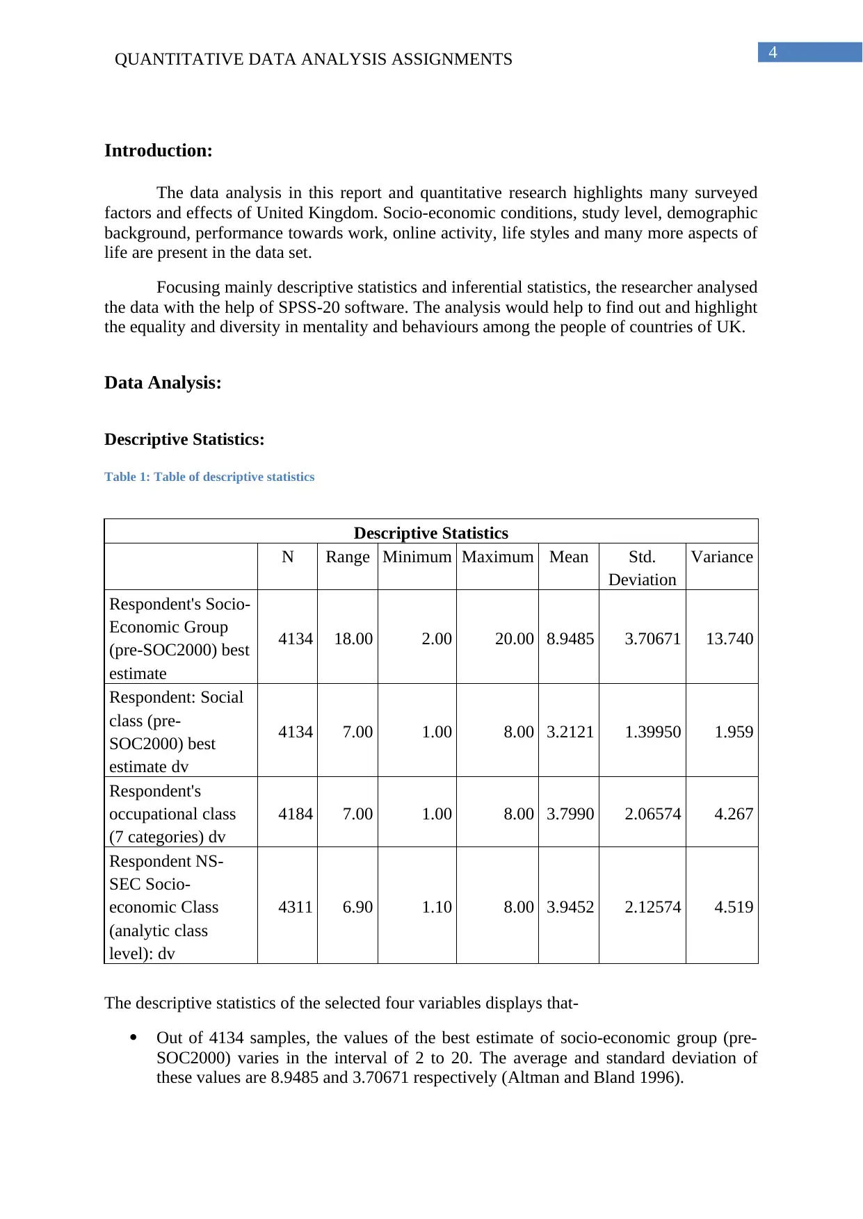
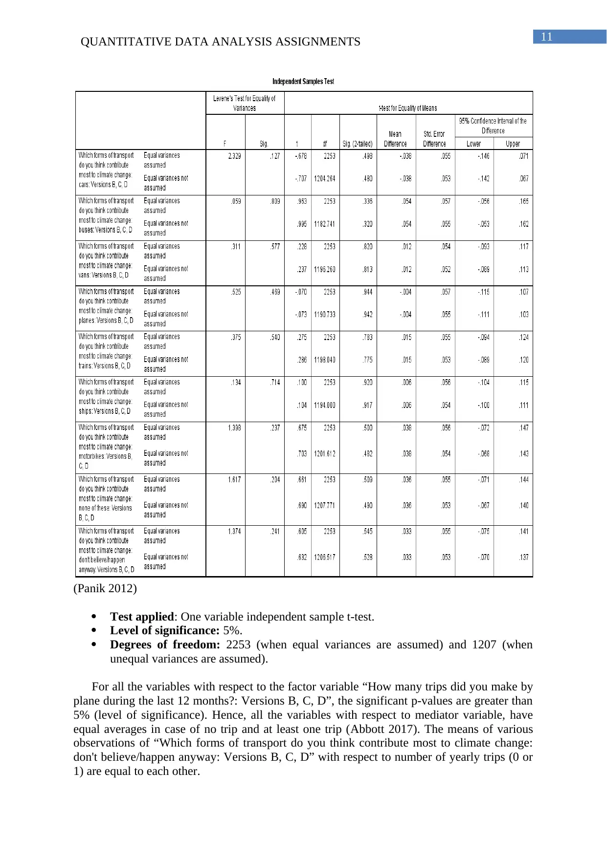
This report presents a quantitative data analysis of the UK Social Attitudes Survey, focusing on socio-economic conditions, study level, demographic backgrounds, work performance, online activity, and lifestyles within the UK. The analysis utilizes descriptive and inferential statistics, employing SPSS-20 software to explore equality and diversity in attitudes and behaviors. The report includes descriptive statistics such as mean and standard deviation for variables like socio-economic group and social class, visualized through box plots to identify outliers. Inferential statistics include paired two-sample t-tests to compare news website preferences, independent sample t-tests to assess the impact of travel frequency on climate change perceptions, Pearson’s correlation coefficient to measure the relationship between urban/rural indicators, Chi-square tests to examine associations between internet access and Twitter usage, one-way ANOVA to compare retired ages across different countries, MANOVA to analyze multivariate effects, and a multiple regression model to predict outcomes. The conclusion summarizes the findings for a lay audience and discusses the limitations of the study. Desklib offers a wealth of similar solved assignments and study resources to aid students in their academic pursuits.

Running head: QUANTITATIVE DATA ANALYSIS ASSIGNMENTS
Quantitative Data Analysis Assignments
Name of the Student:
Name of the University:
Author’s Note:

1QUANTITATIVE DATA ANALYSIS ASSIGNMENTS
Table of Contents
Introduction:...............................................................................................................................2
Data Analysis:............................................................................................................................2
Descriptive Statistics:.............................................................................................................2
Box-plot:................................................................................................................................3
Paired two-sample t-test:........................................................................................................5
Independent sample t-test:......................................................................................................7
Parametric:...........................................................................................................................10
Pearson’s correlation coefficient:.....................................................................................10
Non-Parametric:...................................................................................................................10
Chi-square test:.................................................................................................................10
One-way ANOVA:...............................................................................................................12
MANOVA:...........................................................................................................................14
Multiple Regression Model:.................................................................................................18
Conclusion and Limitations:....................................................................................................22
Reference:................................................................................................................................23

2QUANTITATIVE DATA ANALYSIS ASSIGNMENTS
Table of Tables
Table 1: Table of descriptive statistics.......................................................................................3
Table 2: Tables of paired two-sample t-test...............................................................................6
Table 3: Table of independent sample t-test..............................................................................8
Table 4: Table of Pearson’s correlation coefficient.................................................................11
Table 5: The One-way ANOVA table.....................................................................................13
Table 6: The table of multiple comparisons.............................................................................14
Table 7: Table of Homogeneous subsets.................................................................................15
Table 8: Table of descriptive analysis of MANOVA analysis................................................16
Table 9: Fixed and random effect of multivariate tests of MANOVA analysis......................16
Table 10: Table of testing between-subject effects..................................................................16
Table 11: Table of comparison of Person’s age last birthday with respect to Person 1 sex for
“Males”....................................................................................................................................18
Table 12: Table of Multivariate test of homogeneity...............................................................18
Table 13: Table of Univariate Tests.........................................................................................18
Table 14: Table of Multiple R-square......................................................................................19
Table 15: ANOVA table of multiple regression model...........................................................20
Table 16: Table of intercept and slopes of multiple regression model....................................20
Table of Figures
Figure 1: Distribution of the variable “Respondent’s Socio-Economic Group (pre-SOC2000)
best estimate”.............................................................................................................................5
Figure 2: Distribution of the variable “Respondent’s Social Class (pre-SOC2000) best
estimate”.....................................................................................................................................5

3QUANTITATIVE DATA ANALYSIS ASSIGNMENTS
Figure 3: Distribution of the variable “Respondent’s Occupational Class (7 categories)”........6
Figure 4: The distribution of “Respondent NS-SEC Socio-economic Class” at analytic class
level............................................................................................................................................6
Figure 5: The grouped bar plot of selected two variables........................................................14
Figure 6: The histogram plot of residual values of the multiple regression model..................23
Figure 7: The normal probability plot of standardized residual of multiple regression model23

4QUANTITATIVE DATA ANALYSIS ASSIGNMENTS
Introduction:
The data analysis in this report and quantitative research highlights many surveyed
factors and effects of United Kingdom. Socio-economic conditions, study level, demographic
background, performance towards work, online activity, life styles and many more aspects of
life are present in the data set.
Focusing mainly descriptive statistics and inferential statistics, the researcher analysed
the data with the help of SPSS-20 software. The analysis would help to find out and highlight
the equality and diversity in mentality and behaviours among the people of countries of UK.
Data Analysis:
Descriptive Statistics:
Table 1: Table of descriptive statistics
Descriptive Statistics
N Range Minimum Maximum Mean Std.
Deviation
Variance
Respondent's Socio-
Economic Group
(pre-SOC2000) best
estimate
4134 18.00 2.00 20.00 8.9485 3.70671 13.740
Respondent: Social
class (pre-
SOC2000) best
estimate dv
4134 7.00 1.00 8.00 3.2121 1.39950 1.959
Respondent's
occupational class
(7 categories) dv
4184 7.00 1.00 8.00 3.7990 2.06574 4.267
Respondent NS-
SEC Socio-
economic Class
(analytic class
level): dv
4311 6.90 1.10 8.00 3.9452 2.12574 4.519
The descriptive statistics of the selected four variables displays that-
 Out of 4134 samples, the values of the best estimate of socio-economic group (pre-
SOC2000) varies in the interval of 2 to 20. The average and standard deviation of
these values are 8.9485 and 3.70671 respectively (Altman and Bland 1996).

5QUANTITATIVE DATA ANALYSIS ASSIGNMENTS
 Out of chosen 4134 samples, the values of the best estimate of social class of
respondents varies in the interval of 1 to 8 with range 7. The mean and standard
deviation of these values are 3.2121 and 1.39950.
 Respondent’s occupational class for 4184 samples displays that the highest and lowest
values are 1 and 8 respectively with range 7. The average and standard deviation of
the values of these variables are respectively 3.7990 and 2.06574.
 Respondent NS-SEC Socio-economic class for 4311 samples indicates that the
highest and lowest values are respectively 1.1 and 8. The mean value and standard
deviation of the variable is calculated as 3.9452 and 2.12574.
Box-plot:
Figure 1: Distribution of the variable “Respondent’s Socio-Economic Group (pre-SOC2000) best estimate”
Most of values of the variable (75%) lie in the range of 12 to 7 (Wonnacott and Wonnacott
1990). The median value of the samples is 9. The outliers are the values equal to 20. The
outliers are 716, 900, 897 and 1013th samples (George and Mallery 2016).
Figure 2: Distribution of the variable “Respondent’s Social Class (pre-SOC2000) best estimate”

6QUANTITATIVE DATA ANALYSIS ASSIGNMENTS
Most of values of the variable (75%) lie in the range of 2 to 4. Median is calculated as 3. The
outliers are the values equal to 8. The outliers are 716, 900, 897 and 1013th samples.
Figure 3: Distribution of the variable “Respondent’s Occupational Class (7 categories)”
Most of the values of the variable (75%) lie in the interval of 2 to 6. The median value is
calculated as 3. No outlier is observed in the distribution of the undertaken variable.
Figure 4: The distribution of “Respondent NS-SEC Socio-economic Class” at analytic class level.

7QUANTITATIVE DATA ANALYSIS ASSIGNMENTS
Most of the values of the variable (75%) lie in the interval of 2 to 6. The median value is
calculated as 4. No outlier is observed in the distribution of the chosen variable.
Paired two-sample t-test:
Hypothesis:
Null hypothesis (H0): The average values of two variables “Which news website do you visit
more often” and “Which news website do you visit next more often” are equal to each other.
Alternative hypothesis (HA): The difference of average values of two variables “Which news
website do you visit more often” and “Which news website do you visit more often” is not
equal to 0.
Table 2: Tables of paired two-sample t-test

8QUANTITATIVE DATA ANALYSIS ASSIGNMENTS
The average value of the first variable “Which news website do you visit most often”
is 15.01 for 2268 samples. The average value of the second variable “Which news website do
you visit next most often” is 15.16 for 2268 samples.
 Test applied: Paired two-sample t-test.
 Correlation coefficient: 0.49 with significant p-value 0.019.
 Level of significance: 0.05.
 Degrees of freedom: 2267
 Calculated t-statistic: (-0.172)
 Significant p-value: 0.864.
 Inference: The significant p-value 0.0864 is greater than 0.05. Therefore, the null
hypothesis is not rejected (Traitler Coleman and Burbidge 2017).

9QUANTITATIVE DATA ANALYSIS ASSIGNMENTS
 Interpretation: As the null hypothesis is failed to reject, therefore, it could be
interpreted that the average values of two variables “Which news website do you visit
most often?” and “Which news website do you visit next most often?” are unequal.
 Decision-making: According to the average, the two variables are almost equal to
each other. Therefore, no change would occur significantly in future days in case of
visiting news website (De Winter 2013).
Independent sample t-test:
Null hypothesis (H0): The average values of dependent variable “Which forms of transport
do you think contribute most to climate change: cars: Versions B, C, D” for number of trips 0
or 1 are equal.
Alternative hypothesis (HA): The average values of dependent variable “Which forms of
transport do you think contribute most to climate change: cars: Versions B, C, D” for number
of trips 0 or 1 are unequal.
Table 3: Table of independent sample t-test
Group Statistics
How many trips did you
make by plane during the
last 12 months?: Versions
B, C, D
N Mean Std.
Deviation
Std. Error
Mean
Which forms of
transport do you think
contribute most to
climate change: cars:
Versions B, C, D
0 1639 .78 1.202 .030
1 616 .82 1.096 .044
Which forms of
transport do you think
contribute most to
climate change: buses:
Versions B, C, D
0 1639 .69 1.221 .030
1 616 .63 1.134 .046
Which forms of
transport do you think
contribute most to
climate change: vans:
Versions B, C, D
0 1639 .93 1.159 .029
1 616 .91 1.064 .043
Which forms of
transport do you think
contribute most to
climate change:
planes: Versions B, C,
D
0 1639 .67 1.223 .030
1 616 .68 1.128 .045
Which forms of 0 1639 .21 1.201 .030

10QUANTITATIVE DATA ANALYSIS ASSIGNMENTS
transport do you think
contribute most to
climate change: trains:
Versions B, C, D
1 616 .20 1.101 .044
Which forms of
transport do you think
contribute most to
climate change: ships:
Versions B, C, D
0 1639 .24 1.207 .030
1 616 .24 1.111 .045
Which forms of
transport do you think
contribute most to
climate change:
motorbikes: Versions
B, C, D
0 1639 .25 1.210 .030
1 616 .21 1.106 .045
Which forms of
transport do you think
contribute most to
climate change: none
of these: Versions B,
C, D
0 1639 .17 1.191 .029
1 616 .14 1.082 .044
Which forms of
transport do you think
contribute most to
climate change: don't
believe/happen
anyway: Versions B,
C, D
0 1639 .17 1.191 .029
1 616 .14 1.084 .044

11QUANTITATIVE DATA ANALYSIS ASSIGNMENTS
(Panik 2012)
 Test applied: One variable independent sample t-test.
 Level of significance: 5%.
 Degrees of freedom: 2253 (when equal variances are assumed) and 1207 (when
unequal variances are assumed).
For all the variables with respect to the factor variable “How many trips did you make by
plane during the last 12 months?: Versions B, C, D”, the significant p-values are greater than
5% (level of significance). Hence, all the variables with respect to mediator variable, have
equal averages in case of no trip and at least one trip (Abbott 2017). The means of various
observations of “Which forms of transport do you think contribute most to climate change:
don't believe/happen anyway: Versions B, C, D” with respect to number of yearly trips (0 or
1) are equal to each other.