Quantitative Methods with Economics - Analysis and Computation

This document provides a detailed analysis and computation of quantitative methods with economics. It covers topics such as equilibrium point, profit function, demand and supply function, and more. The document also includes tables and graphs for better understanding. The subject is Quantitative Methods with Economics and the course code is MAT10706.

QUANTITATIVE METHDS WITH ECONOMICS
MAT10706
[Pick the date]
Student Name

Question 1
Part 1
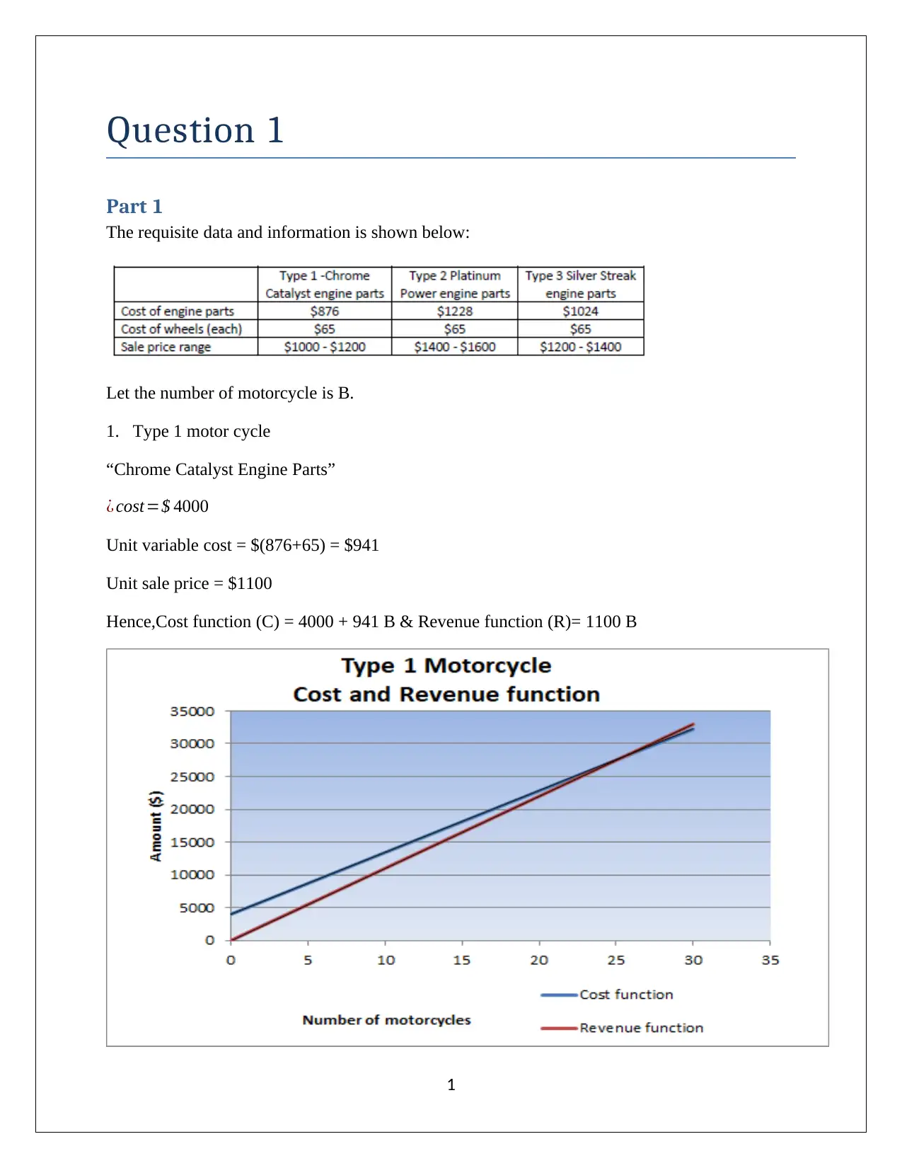
The requisite data and information is shown below:
Let the number of motorcycle is B.
1. Type 1 motor cycle
“Chrome Catalyst Engine Parts”
¿ cost=$ 4000
Unit variable cost = $(876+65) = $941
Unit sale price = $1100
Hence,Cost function (C) = 4000 + 941 B & Revenue function (R)= 1100 B
1

2. Type 2 motor cycle
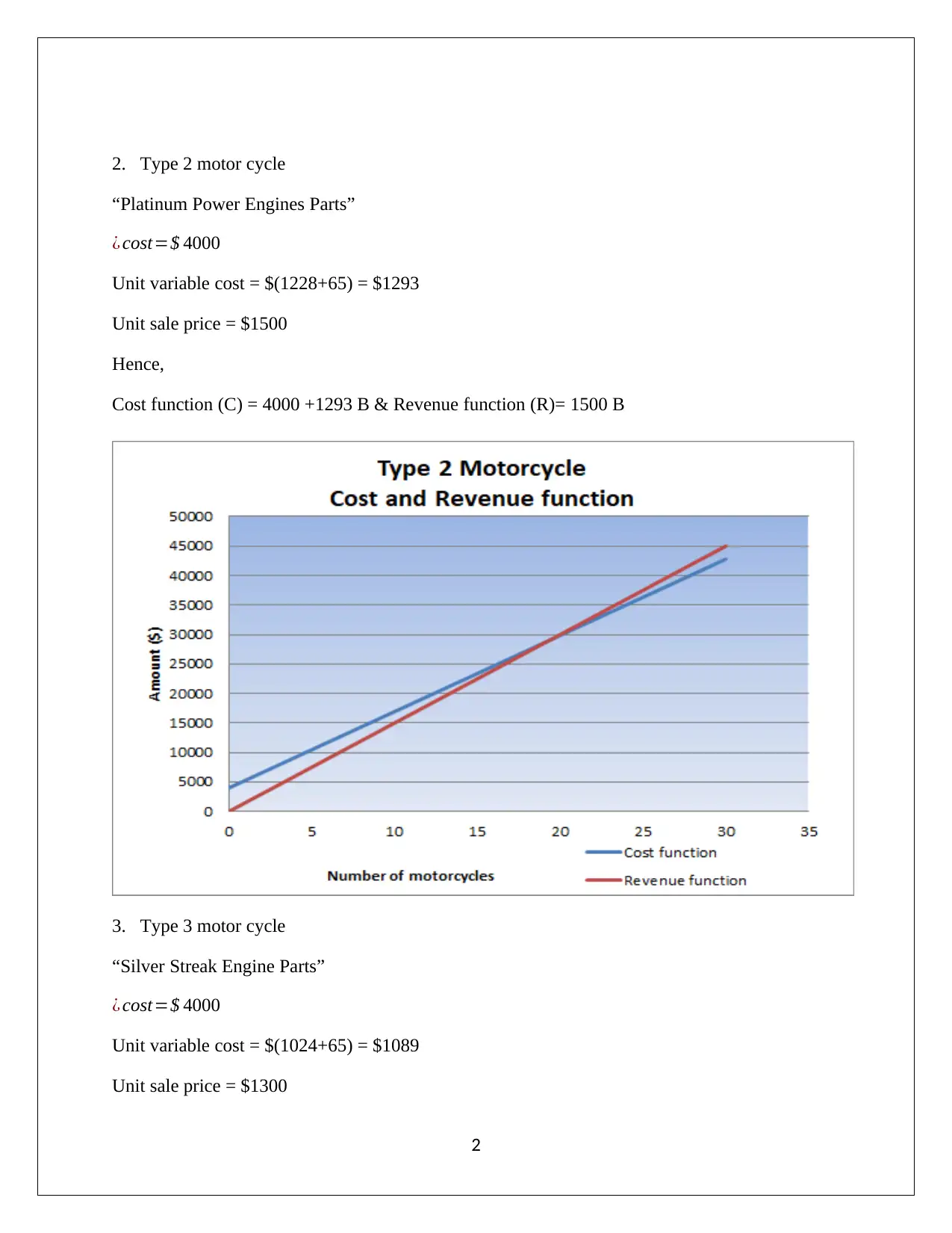
“Platinum Power Engines Parts”
¿ cost=$ 4000
Unit variable cost = $(1228+65) = $1293
Unit sale price = $1500
Hence,
Cost function (C) = 4000 +1293 B & Revenue function (R)= 1500 B
3. Type 3 motor cycle
“Silver Streak Engine Parts”
¿ cost=$ 4000
Unit variable cost = $(1024+65) = $1089
Unit sale price = $1300
2

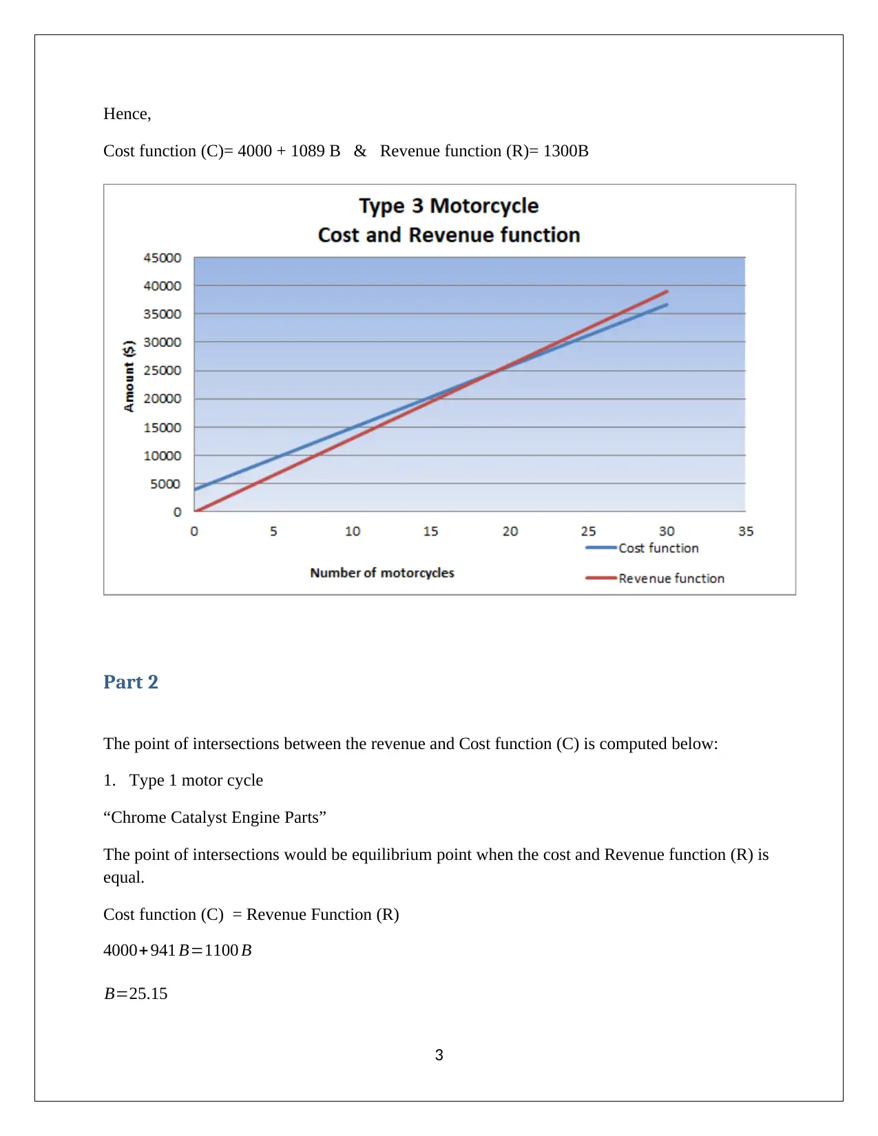
Hence,
Cost function (C)= 4000 + 1089 B & Revenue function (R)= 1300B
Part 2
The point of intersections between the revenue and Cost function (C) is computed below:
1. Type 1 motor cycle
“Chrome Catalyst Engine Parts”
The point of intersections would be equilibrium point when the cost and Revenue function (R) is
equal.
Cost function (C) = Revenue Function (R)
4000+ 941 B=1100 B
B=25.15
3

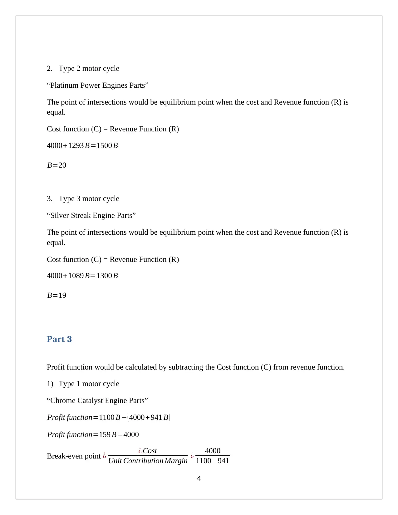
2. Type 2 motor cycle
“Platinum Power Engines Parts”
The point of intersections would be equilibrium point when the cost and Revenue function (R) is
equal.
Cost function (C) = Revenue Function (R)
4000+ 1293 B=1500 B
B=20
3. Type 3 motor cycle
“Silver Streak Engine Parts”
The point of intersections would be equilibrium point when the cost and Revenue function (R) is
equal.
Cost function (C) = Revenue Function (R)
4000+ 1089 B=1300 B
B=19
Part 3
Profit function would be calculated by subtracting the Cost function (C) from revenue function.
1) Type 1 motor cycle
“Chrome Catalyst Engine Parts”
Profit function=1100 B− ( 4000+ 941 B )
Profit function=159 B – 4000
Break-even point ¿ ¿ Cost
Unit Contribution Margin ¿ 4000
1100−941
4

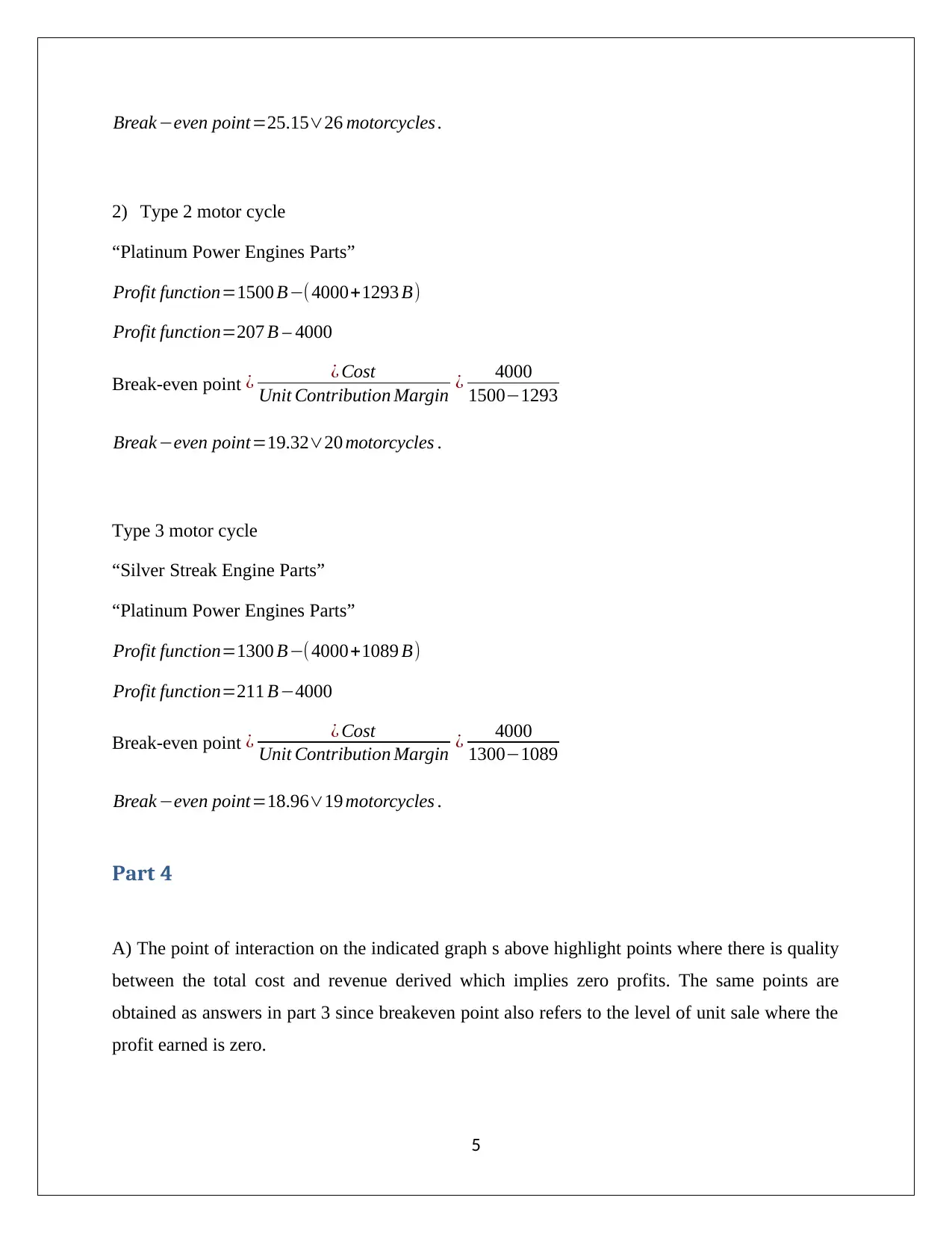
Break−even point=25.15∨26 motorcycles .
2) Type 2 motor cycle
“Platinum Power Engines Parts”
Profit function=1500 B−(4000+1293 B)
Profit function=207 B – 4000
Break-even point ¿ ¿ Cost
Unit Contribution Margin ¿ 4000
1500−1293
Break−even point=19.32∨20 motorcycles .
Type 3 motor cycle
“Silver Streak Engine Parts”
“Platinum Power Engines Parts”
Profit function=1300 B−(4000+1089 B)
Profit function=211 B−4000
Break-even point ¿ ¿ Cost
Unit Contribution Margin ¿ 4000
1300−1089
Break −even point=18.96∨19 motorcycles .
Part 4
A) The point of interaction on the indicated graph s above highlight points where there is quality
between the total cost and revenue derived which implies zero profits. The same points are
obtained as answers in part 3 since breakeven point also refers to the level of unit sale where the
profit earned is zero.
5

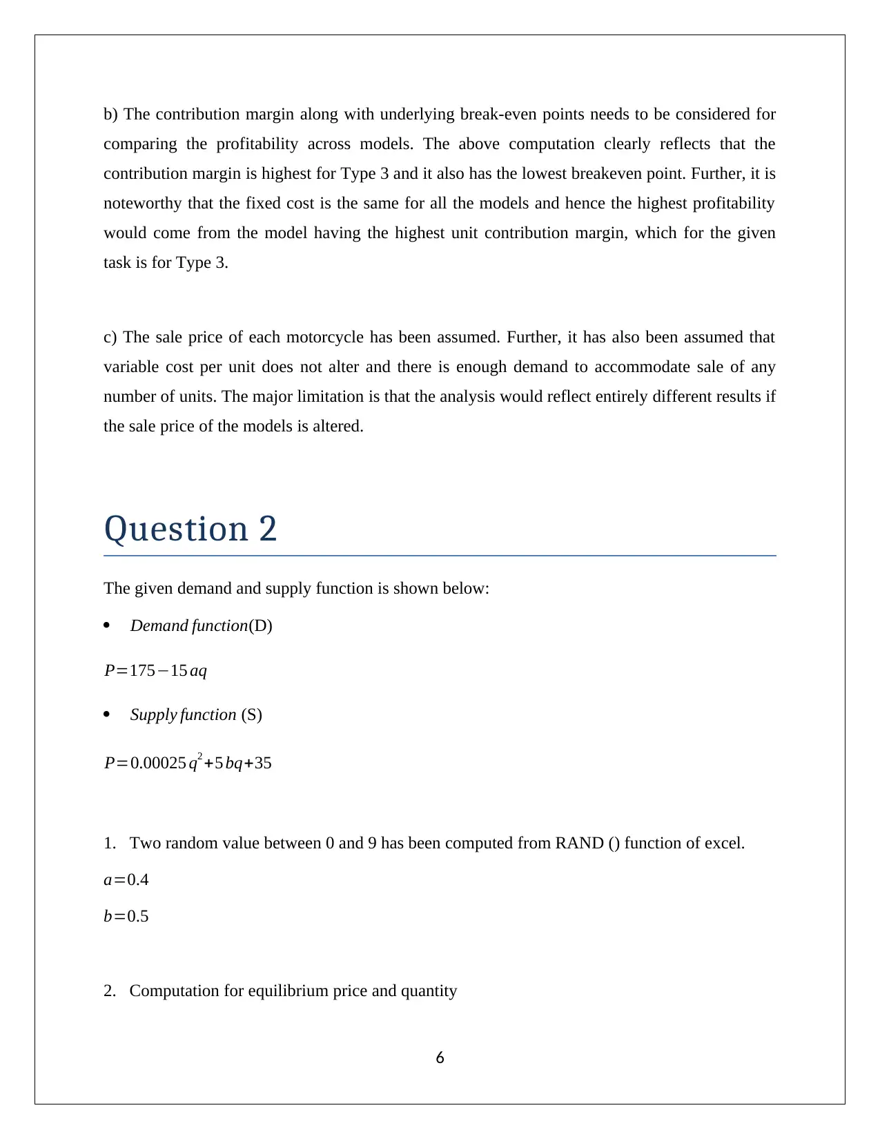
b) The contribution margin along with underlying break-even points needs to be considered for
comparing the profitability across models. The above computation clearly reflects that the
contribution margin is highest for Type 3 and it also has the lowest breakeven point. Further, it is
noteworthy that the fixed cost is the same for all the models and hence the highest profitability
would come from the model having the highest unit contribution margin, which for the given
task is for Type 3.
c) The sale price of each motorcycle has been assumed. Further, it has also been assumed that
variable cost per unit does not alter and there is enough demand to accommodate sale of any
number of units. The major limitation is that the analysis would reflect entirely different results if
the sale price of the models is altered.
Question 2
The given demand and supply function is shown below:
 Demand function(D)
P=175−15 aq
 Supply function (S)
P=0.00025 q2 +5 bq+35
1. Two random value between 0 and 9 has been computed from RAND () function of excel.
a=0.4
b=0.5
2. Computation for equilibrium price and quantity
6

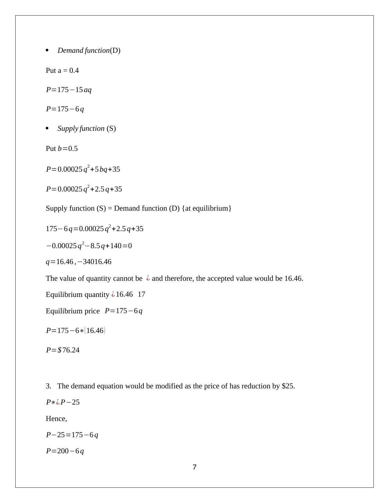
 Demand function(D)
Put a = 0.4
P=175−15 aq
P=175−6 q
 Supply function (S)
Put b=0.5
P=0.00025 q2 +5 bq+35
P=0.00025 q2 +2.5 q+35
Supply function (S) = Demand function (D) {at equilibrium}
175−6 q=0.00025 q2 +2.5 q+35
−0.00025 q2−8.5 q+140=0
q=16.46 ,−34016.46
The value of quantity cannot be ¿ and therefore, the accepted value would be 16.46.
Equilibrium quantity ¿ 16.46 17
Equilibrium price P=175−6 q
P=175−6∗( 16.46 )
P=$ 76.24
3. The demand equation would be modified as the price of has reduction by $25.
P∗¿ P−25
Hence,
P−25=175−6 q
P=200−6 q
7

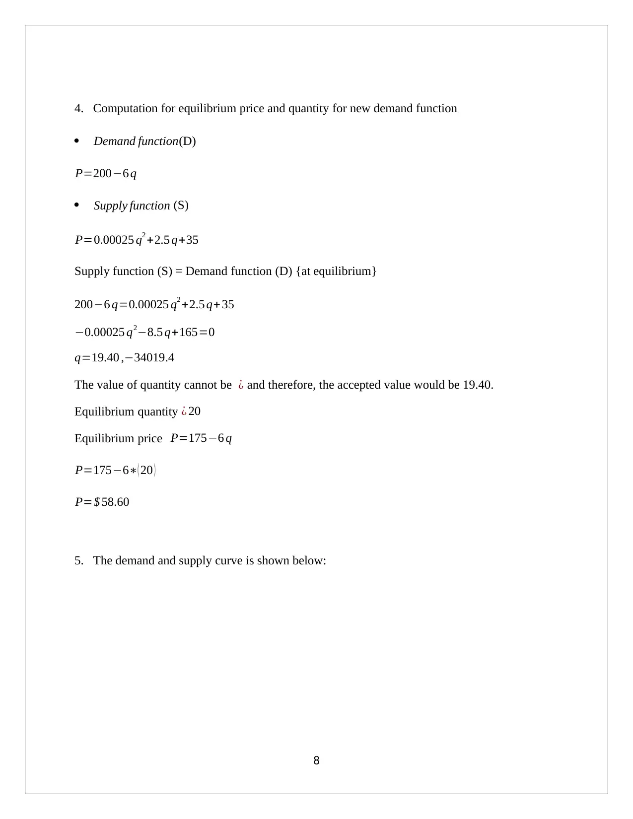
4. Computation for equilibrium price and quantity for new demand function
 Demand function(D)
P=200−6 q
 Supply function (S)
P=0.00025 q2 +2.5 q+35
Supply function (S) = Demand function (D) {at equilibrium}
200−6 q=0.00025 q2 +2.5 q+ 35
−0.00025 q2−8.5 q+165=0
q=19.40 ,−34019.4
The value of quantity cannot be ¿ and therefore, the accepted value would be 19.40.
Equilibrium quantity ¿ 20
Equilibrium price P=175−6 q
P=175−6∗( 20 )
P=$ 58.60
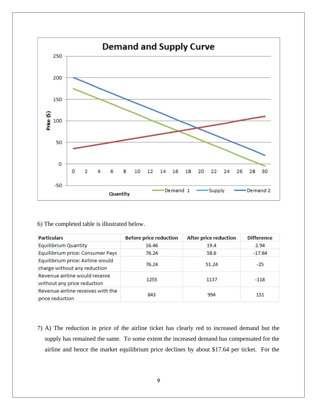
5. The demand and supply curve is shown below:
8

6) The completed table is illustrated below.
7) A) The reduction in price of the airline ticket has clearly red to increased demand but the
supply has remained the same. To some extent the increased demand has compensated for the
airline and hence the market equilibrium price declines by about $17.64 per ticket. For the
9

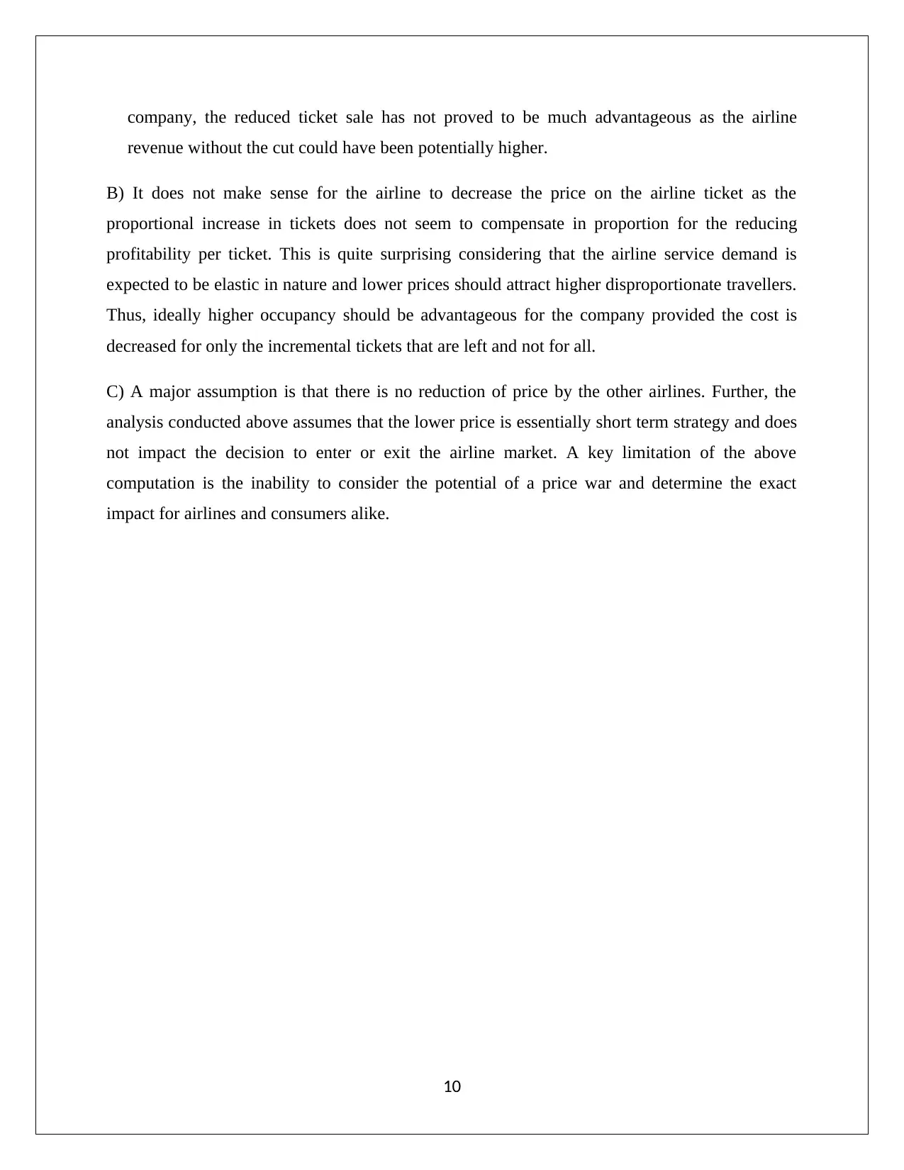
company, the reduced ticket sale has not proved to be much advantageous as the airline
revenue without the cut could have been potentially higher.
B) It does not make sense for the airline to decrease the price on the airline ticket as the
proportional increase in tickets does not seem to compensate in proportion for the reducing
profitability per ticket. This is quite surprising considering that the airline service demand is
expected to be elastic in nature and lower prices should attract higher disproportionate travellers.
Thus, ideally higher occupancy should be advantageous for the company provided the cost is
decreased for only the incremental tickets that are left and not for all.
C) A major assumption is that there is no reduction of price by the other airlines. Further, the
analysis conducted above assumes that the lower price is essentially short term strategy and does
not impact the decision to enter or exit the airline market. A key limitation of the above
computation is the inability to consider the potential of a price war and determine the exact
impact for airlines and consumers alike.
10