Bivariate Linear Regression Model

This document discusses the bivariate linear regression model for demand and price of coffee. It includes a plot showing the relationship between demand and price, as well as regression statistics and coefficients.

Quantitative methods

Contents
Section (A): Bivariate Linear Regression Model.....................................................................................3
1) Plot..................................................................................................................................................3
Section B Multivariate Regression Analysis............................................................................................7
Section (C) Coefficient of Variation.........................................................................................................9
REFERENCES........................................................................................................................................10

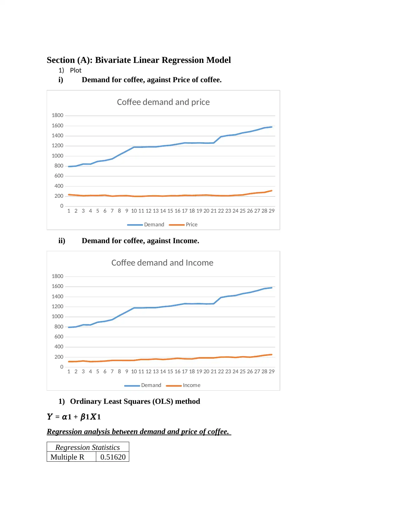
Section (A): Bivariate Linear Regression Model
1) Plot
i) Demand for coffee, against Price of coffee.
1 2 3 4 5 6 7 8 9 10 11 12 13 14 15 16 17 18 19 20 21 22 23 24 25 26 27 28 29
0
200
400
600
800
1000
1200
1400
1600
1800
Coffee demand and price
Demand Price
ii) Demand for coffee, against Income.
1 2 3 4 5 6 7 8 9 10 11 12 13 14 15 16 17 18 19 20 21 22 23 24 25 26 27 28 29
0
200
400
600
800
1000
1200
1400
1600
1800
Coffee demand and Income
Demand Income
1) Ordinary Least Squares (OLS) method
𝑌 = 𝛼1 + 𝛽1𝑋1
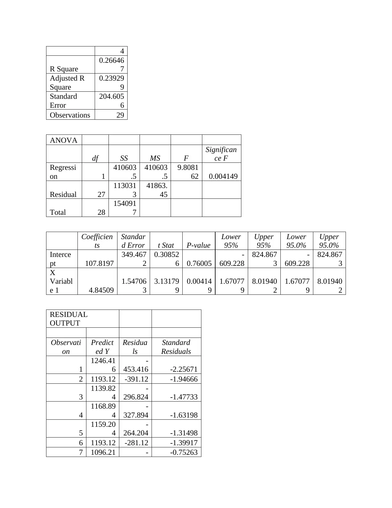
Regression analysis between demand and price of coffee.
Regression Statistics
Multiple R 0.51620

4
R Square
0.26646
7
Adjusted R
Square
0.23929
9
Standard
Error
204.605
6
Observations 29
ANOVA
df SS MS F
Significan
ce F
Regressi
on 1
410603
.5
410603
.5
9.8081
62 0.004149
Residual 27
113031
3
41863.
45
Total 28
154091
7
Coefficien
ts
Standar
d Error t Stat P-value
Lower
95%
Upper
95%
Lower
95.0%
Upper
95.0%
Interce
pt 107.8197
349.467
2
0.30852
6 0.76005
-
609.228
824.867
3
-
609.228
824.867
3
X
Variabl
e 1 4.84509
1.54706
3
3.13179
9
0.00414
9
1.67077
9
8.01940
2
1.67077
9
8.01940
2
RESIDUAL
OUTPUT
Observati
on
Predict
ed Y
Residua
ls
Standard
Residuals
1
1246.41
6
-
453.416 -2.25671
2 1193.12 -391.12 -1.94666
3
1139.82
4
-
296.824 -1.47733
4
1168.89
4
-
327.894 -1.63198
5
1159.20
4
-
264.204 -1.31498
6 1193.12 -281.12 -1.39917
7 1096.21 - -0.75263

8 151.218
8
1139.82
4
-
112.824 -0.56154
9
1149.51
4
-
48.5141 -0.24146
10
1081.68
3
97.3171
3 0.484361
11
1076.83
8
102.162
2 0.508475
12
1115.59
9 68.4015 0.340444
13
1125.28
9
58.7113
1 0.292214
14
1101.06
3
100.936
8 0.502376
15
1139.82
4
75.1760
4 0.374161
16
1134.97
9
103.021
1 0.51275
17
1178.58
5
84.4153
2 0.420147
18
1164.04
9
95.9505
9 0.477559
19
1188.27
5
74.7251
4 0.371917
20
1207.65
5
50.3447
8 0.250573
21
1164.04
9
96.9505
9 0.482536
22
1139.82
4 246.176 1.225252
23
1134.97
9
276.021
1 1.373795
24 1183.43
241.570
2 1.202328
25
1217.34
5
244.654
6 1.217679
26
1333.62
8
152.372
4 0.758378
27
1415.99
4
105.005
9 0.522629
28
1464.44
5
98.5549
9 0.490522
29
1624.33
3 -45.333 -0.22563

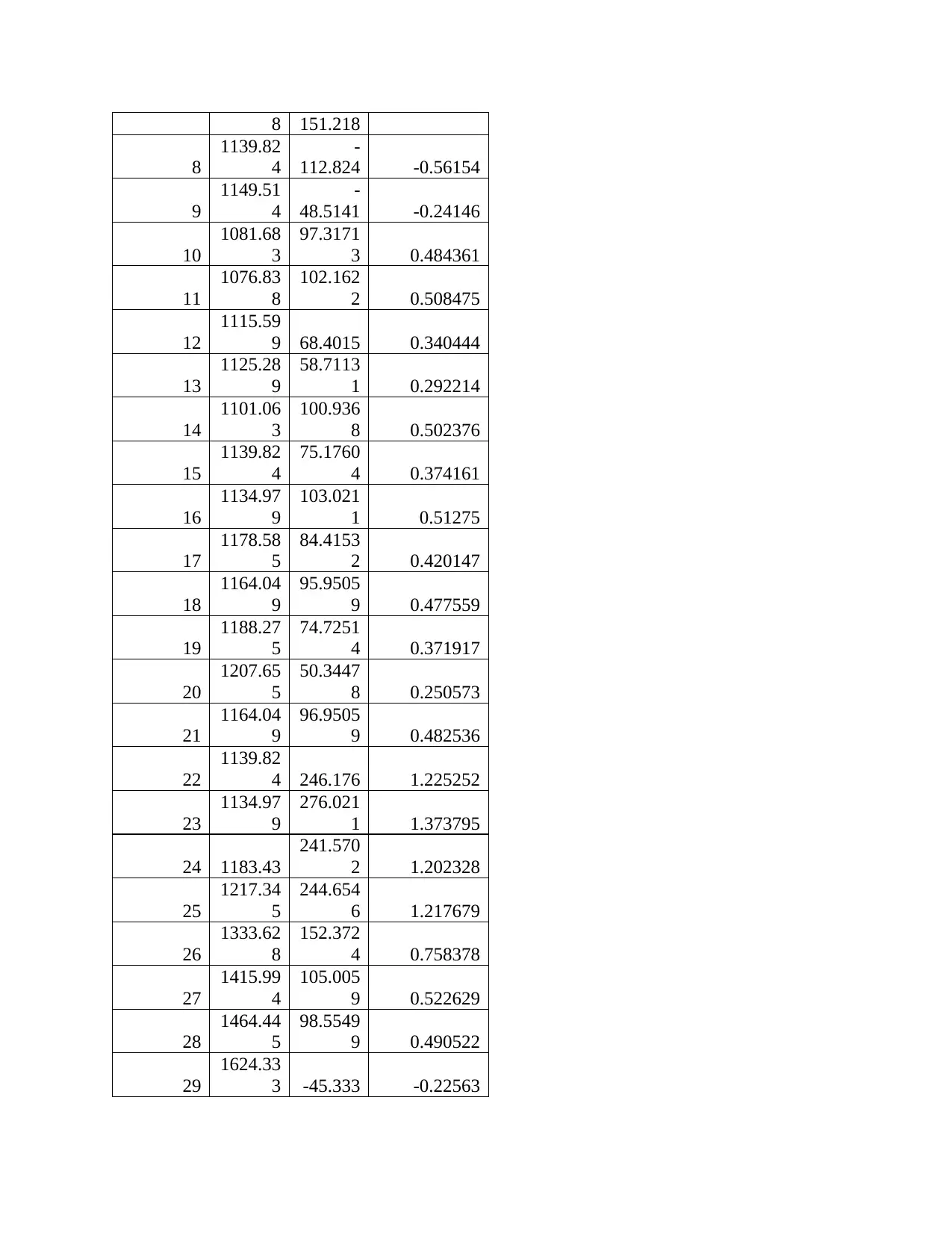
2) Coefficient of determination
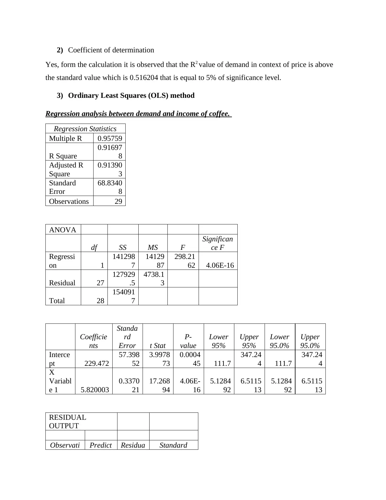
Yes, form the calculation it is observed that the R2 value of demand in context of price is above
the standard value which is 0.516204 that is equal to 5% of significance level.
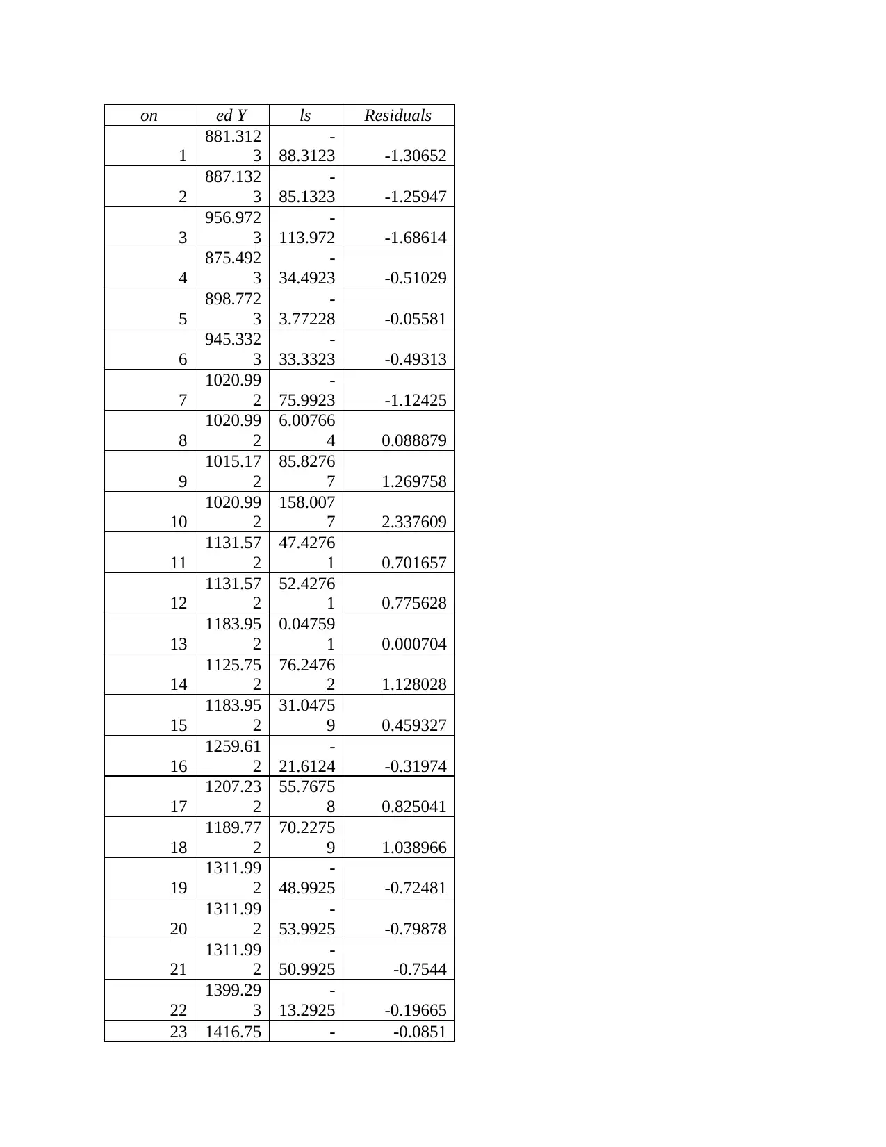
3) Ordinary Least Squares (OLS) method
Regression analysis between demand and income of coffee.
Regression Statistics
Multiple R 0.95759
R Square
0.91697
8
Adjusted R
Square
0.91390
3
Standard
Error
68.8340
8
Observations 29
ANOVA
df SS MS F
Significan
ce F
Regressi
on 1
141298
7
14129
87
298.21
62 4.06E-16
Residual 27
127929
.5
4738.1
3
Total 28
154091
7
Coefficie
nts
Standa
rd
Error t Stat
P-
value
Lower
95%
Upper
95%
Lower
95.0%
Upper
95.0%
Interce
pt 229.472
57.398
52
3.9978
73
0.0004
45 111.7
347.24
4 111.7
347.24
4
X
Variabl
e 1 5.820003
0.3370
21
17.268
94
4.06E-
16
5.1284
92
6.5115
13
5.1284
92
6.5115
13
RESIDUAL
OUTPUT
Observati Predict Residua Standard

on ed Y ls Residuals
1
881.312
3
-
88.3123 -1.30652
2
887.132
3
-
85.1323 -1.25947
3
956.972
3
-
113.972 -1.68614
4
875.492
3
-
34.4923 -0.51029
5
898.772
3
-
3.77228 -0.05581
6
945.332
3
-
33.3323 -0.49313
7
1020.99
2
-
75.9923 -1.12425
8
1020.99
2
6.00766
4 0.088879
9
1015.17
2
85.8276
7 1.269758
10
1020.99
2
158.007
7 2.337609
11
1131.57
2
47.4276
1 0.701657
12
1131.57
2
52.4276
1 0.775628
13
1183.95
2
0.04759
1 0.000704
14
1125.75
2
76.2476
2 1.128028
15
1183.95
2
31.0475
9 0.459327
16
1259.61
2
-
21.6124 -0.31974
17
1207.23
2
55.7675
8 0.825041
18
1189.77
2
70.2275
9 1.038966
19
1311.99
2
-
48.9925 -0.72481
20
1311.99
2
-
53.9925 -0.79878
21
1311.99
2
-
50.9925 -0.7544
22
1399.29
3
-
13.2925 -0.19665
23 1416.75 - -0.0851

3 5.75251
24
1358.55
2
66.4475
1 0.983043
25
1440.03
3
21.9674
8 0.324993
26
1393.47
3 92.5275 1.368877
27
1486.59
3
34.4074
6 0.509033
28
1614.63
3
-
51.6326 -0.76387
29
1696.11
3
-
117.113 -1.7326
4) Coefficient of determination
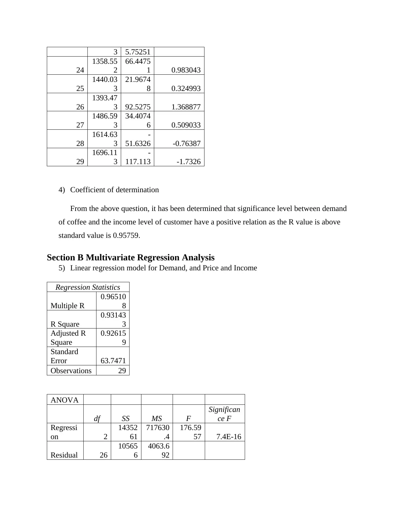
From the above question, it has been determined that significance level between demand
of coffee and the income level of customer have a positive relation as the R value is above
standard value is 0.95759.
Section B Multivariate Regression Analysis
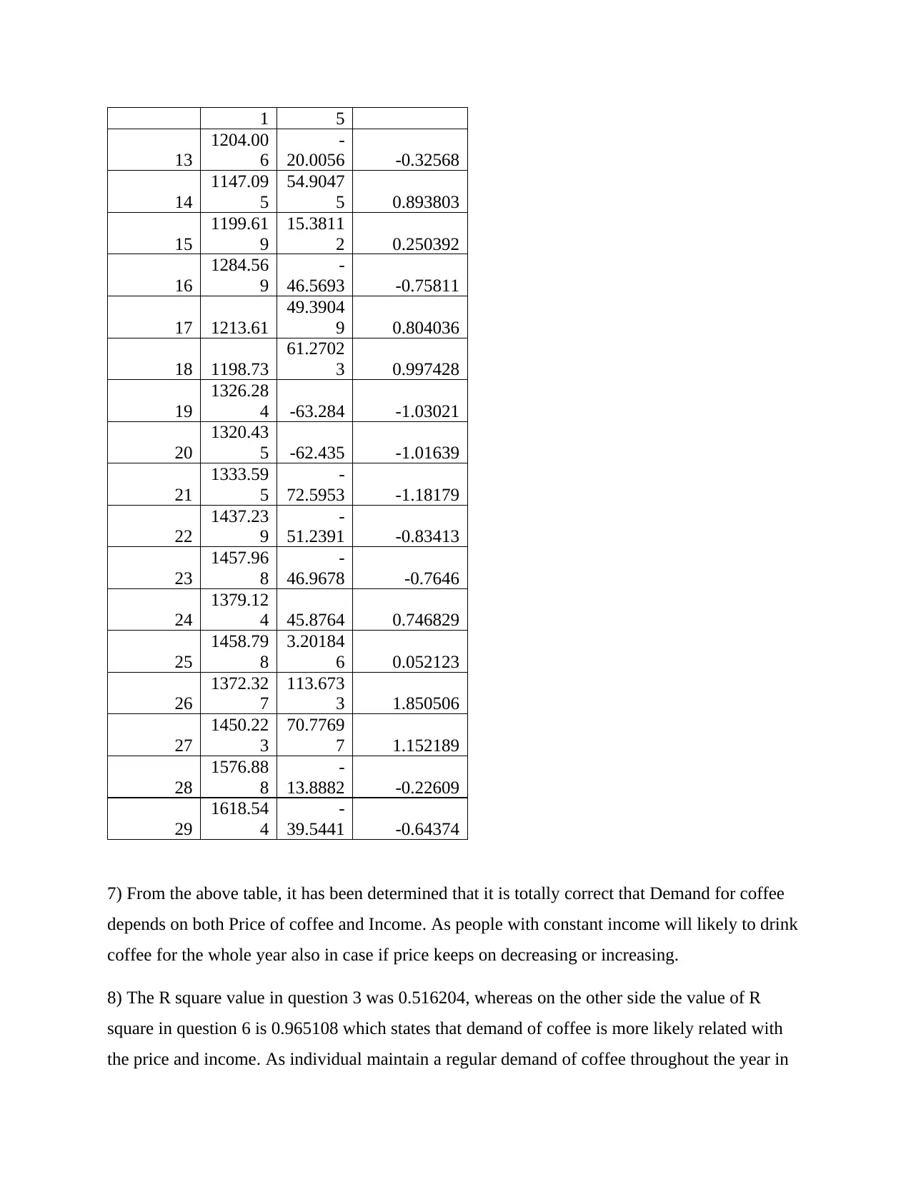
5) Linear regression model for Demand, and Price and Income
Regression Statistics
Multiple R
0.96510
8
R Square
0.93143
3
Adjusted R
Square
0.92615
9
Standard
Error 63.7471
Observations 29
ANOVA
df SS MS F
Significan
ce F
Regressi
on 2
14352
61
717630
.4
176.59
57 7.4E-16
Residual 26
10565
6
4063.6
92

Total 28
15409
17
Coefficie
nts
Standa
rd
Error t Stat
P-
value
Lower
95%
Upper
95%
Lower
95.0%
Upper
95.0%
Interce
pt 457.8438
111.08
92
4.1214
07
0.0003
4
229.49
67
686.19
09
229.49
67
686.19
09
X
Variabl
e 1 6.422167
0.4044
39
15.879
21
6.75E-
15
5.5908
31
7.2535
03
5.5908
31
7.2535
03
X
Variabl
e 2 -1.46226
0.6245
82
-
2.3411
8
0.0271
64 -2.7461
-
0.1784
1 -2.7461
-
0.1784
1
RESIDUAL
OUTPUT
Observati
on
Predict
ed Y
Residua
ls
Standard
Residuals
1
833.496
6
-
40.4966 -0.65925
2
856.003
6
-
54.0036 -0.87913
3
949.154
4
-
106.154 -1.7281
4
850.470
5
-
9.47049 -0.15417
5
879.083
7
15.9163
3 0.259104
6
920.225
2
-
8.22522 -0.1339
7
1032.95
8
-
87.9585 -1.43189
8
1019.79
8
7.20179
7 0.117239
9
1010.45
2
90.5484
7 1.474053
10
1037.34
5
141.654
7 2.30602
11
1160.82
9
18.1713
1 0.295814
12 1149.13 34.8693 0.567644

1 5
13
1204.00
6
-
20.0056 -0.32568
14
1147.09
5
54.9047
5 0.893803
15
1199.61
9
15.3811
2 0.250392
16
1284.56
9
-
46.5693 -0.75811
17 1213.61
49.3904
9 0.804036
18 1198.73
61.2702
3 0.997428
19
1326.28
4 -63.284 -1.03021
20
1320.43
5 -62.435 -1.01639
21
1333.59
5
-
72.5953 -1.18179
22
1437.23
9
-
51.2391 -0.83413
23
1457.96
8
-
46.9678 -0.7646
24
1379.12
4 45.8764 0.746829
25
1458.79
8
3.20184
6 0.052123
26
1372.32
7
113.673
3 1.850506
27
1450.22
3
70.7769
7 1.152189
28
1576.88
8
-
13.8882 -0.22609
29
1618.54
4
-
39.5441 -0.64374
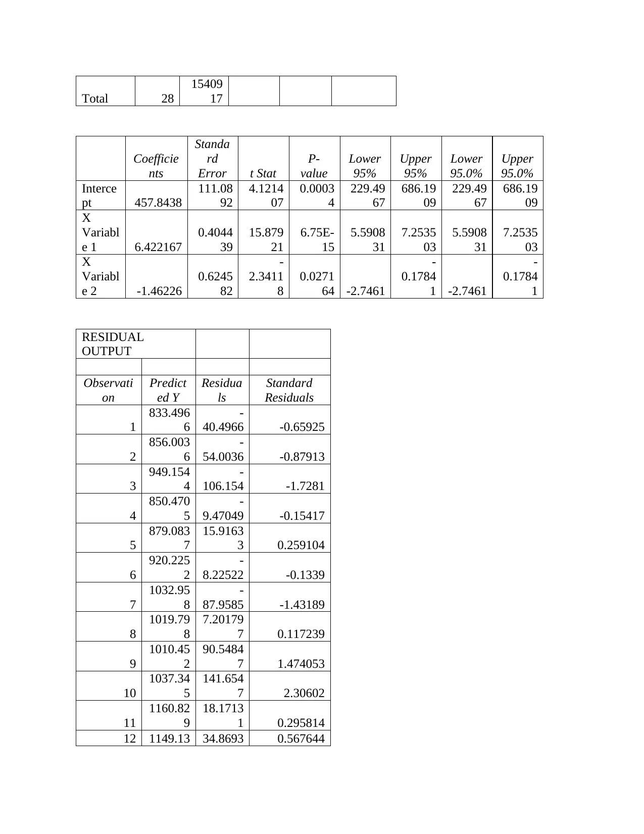
7) From the above table, it has been determined that it is totally correct that Demand for coffee
depends on both Price of coffee and Income. As people with constant income will likely to drink
coffee for the whole year also in case if price keeps on decreasing or increasing.
8) The R square value in question 3 was 0.516204, whereas on the other side the value of R
square in question 6 is 0.965108 which states that demand of coffee is more likely related with
the price and income. As individual maintain a regular demand of coffee throughout the year in

case of price decrease as well as they never give up while drinking coffee in case of price
increase.
9) From the above discussion, it is concluded that regression validation remains the procedure of
determining whether the arithmetical consequences quantifying imagined relations among
variables, found since regression analysis, are satisfactory as accounts of the information. The
endorsement process can contain examining the goodness of appropriate of the deterioration,
examining whether the regression residuals are accidental, and examination whether the
simulation's predictive presentation deteriorates considerably when practical to information that
remained not used in perfect estimation.
10) Two variables instead of price and income which can impact the price of coffee in UK:
 Decrease in prices of Tea: In case if prices of tea decrease people will automatically
switch to alternative product which may impact the demand of coffee.
 Health issues such as sleep difficulty: As people consuming more coffee might face the
issue of improper sleep as coffee contains Nicotine that is not good for health.
Section (C) Coefficient of Variation
11) From the information presented in the question, it is clearly determined that stock of Corvus
Ltd. Is more risk as the value of standard deviation is more as compared to other company which
is Pavo PLC.

REFERENCES
Ndahimana, D. and Kim, E.K., 2017. Measurement methods for physical activity and energy
expenditure: a review. Clinical nutrition research, 6(2), p.68.
Knapp, A.C., 2017. The Effect of Aerobic Exercise Training on Components of Total Energy
Expenditure (Doctoral dissertation, University of South Alabama).
Ranganathan, P., Pramesh, C.S. and Aggarwal, R., 2017. Common pitfalls in statistical analysis:
Measures of agreement. Perspectives in clinical research, 8(4), p.187.
Heydenreich, J., Kayser, B., Schutz, Y. and Melzer, K., 2017. Total energy expenditure, energy
intake, and body composition in endurance athletes across the training season: A
systematic review. Sports medicine-open, 3(1), pp.1-24.