Quantitative Methods in the Social Sciences-SPSS

This document discusses various topics related to quantitative methods in the social sciences using SPSS. It covers distance of sample mean from the population, confidence interval level, null hypothesis and results interpretation, sampling distribution, dependence of the mean and standard deviation in sample distribution, and more.

QUANTITATIVE METHODS IN THE
SOCIAL SCIENCES-SPSS

TABLE OF CONTENTS
(1).....................................................................................................................................................1
(a)Distance of sample mean from the population.......................................................................1
(b) Confidence interval level.......................................................................................................1
© Null hypothesis and results interpretation...............................................................................1
(2).....................................................................................................................................................1
(a)Sampling distribution.............................................................................................................1
(b) Dependence of the mean and standard deviation of varied samples in sample distribution
depend.........................................................................................................................................1
© Reason behind testing of significance when inferring from sample to population.................1
(d and e) Explanation of probability...........................................................................................2
(3).....................................................................................................................................................2
(a)................................................................................................................................................2
(b)................................................................................................................................................2
(4).....................................................................................................................................................3
(5).....................................................................................................................................................4
(a)Discussion of findings............................................................................................................5
(b) Discuss causality...................................................................................................................5
© Testing of model for 10 years later.........................................................................................6
(6).....................................................................................................................................................7
(a)Mean age of passenger............................................................................................................8
(b & c) Reporting of significant difference between class..........................................................8
(7).....................................................................................................................................................8
(a)Proportion of dead and survival in each class........................................................................9
(b) Measure of association between passenger class and survival..............................................9
© Significance of difference.......................................................................................................9
REFERENCES..............................................................................................................................12

(1)
(a)Distance of sample mean from the population
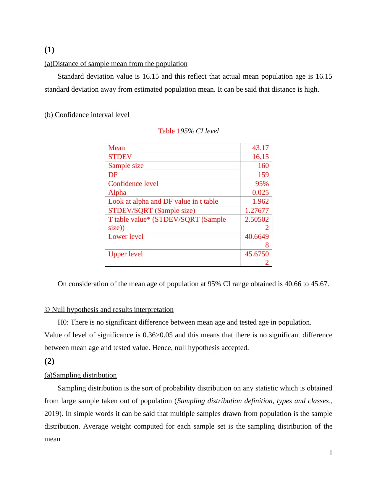
Standard deviation value is 16.15 and this reflect that actual mean population age is 16.15
standard deviation away from estimated population mean. It can be said that distance is high.
(b) Confidence interval level
Table 195% CI level
Mean 43.17
STDEV 16.15
Sample size 160
DF 159
Confidence level 95%
Alpha 0.025
Look at alpha and DF value in t table 1.962
STDEV/SQRT (Sample size) 1.27677
T table value* (STDEV/SQRT (Sample
size))
2.50502
2
Lower level 40.6649
8
Upper level 45.6750
2
On consideration of the mean age of population at 95% CI range obtained is 40.66 to 45.67.
© Null hypothesis and results interpretation
H0: There is no significant difference between mean age and tested age in population.
Value of level of significance is 0.36>0.05 and this means that there is no significant difference
between mean age and tested value. Hence, null hypothesis accepted.
(2)
(a)Sampling distribution
Sampling distribution is the sort of probability distribution on any statistic which is obtained
from large sample taken out of population (Sampling distribution definition, types and classes.,
2019). In simple words it can be said that multiple samples drawn from population is the sample
distribution. Average weight computed for each sample set is the sampling distribution of the
mean
1

(b) Dependence of the mean and standard deviation of varied samples in sample distribution
depend
Mean and standard deviation of sample distribution depend on characteristics of the sample
units in multiple sample and sample size. Important point to note is that many times in varied
researches small sample size is taken whose mean value is different from the other sample with
same characteristics but large sample size (Camilleri, 2017). Thus, it can be said that mean and
standard deviation of sample distribution depend on these two factors.
© Reason behind testing of significance when inferring from sample to population
Main reason behind testing of significance is that every time when research is carried out on
sample there is doubt whether it is actually mirroring population. In case sample does not
actually reflect population then results obtained may be wrong (Williams and Bornmann, 2016).
Hence, testing of significance is done to check whether results obtained from sample are
different or same in respect to population mean and standard deviation.
(d and e) Explanation of probability
It is the probability of occurrence or existence of the alternative hypothesis. For example, in
case of regression we state that we are 95% confident there is significant impact of one variable
on other one. So remaining probability is 5% which reflect that analyst believe that there is 5%
chance that no difference will be observed between variables. If obtained probability is higher
then 5% then this reflect that actually more than 5% like in our case there is chance that there is
no difference between sample mean and tested value. Hence, in present case probability is
0.36>0.05 and this means that probability of no significant difference between actual mean and
tested value is 36% and it is high. Thus, p value in statistical analysis reflect probability of no
significant difference or relationship between variables.
(3)
(a)
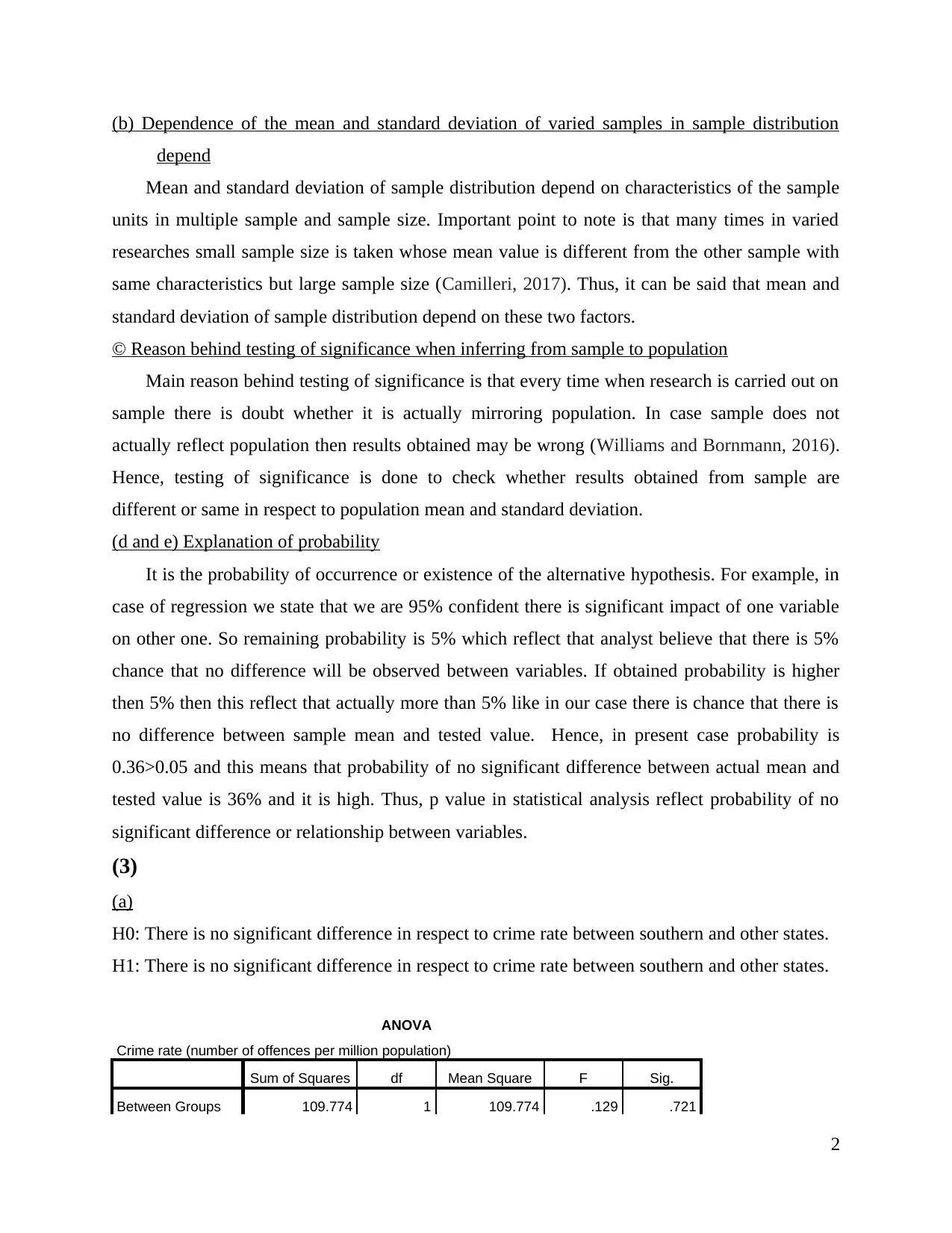
H0: There is no significant difference in respect to crime rate between southern and other states.
H1: There is no significant difference in respect to crime rate between southern and other states.
ANOVA
Crime rate (number of offences per million population)
Sum of Squares df Mean Square F Sig.
Between Groups 109.774 1 109.774 .129 .721
2

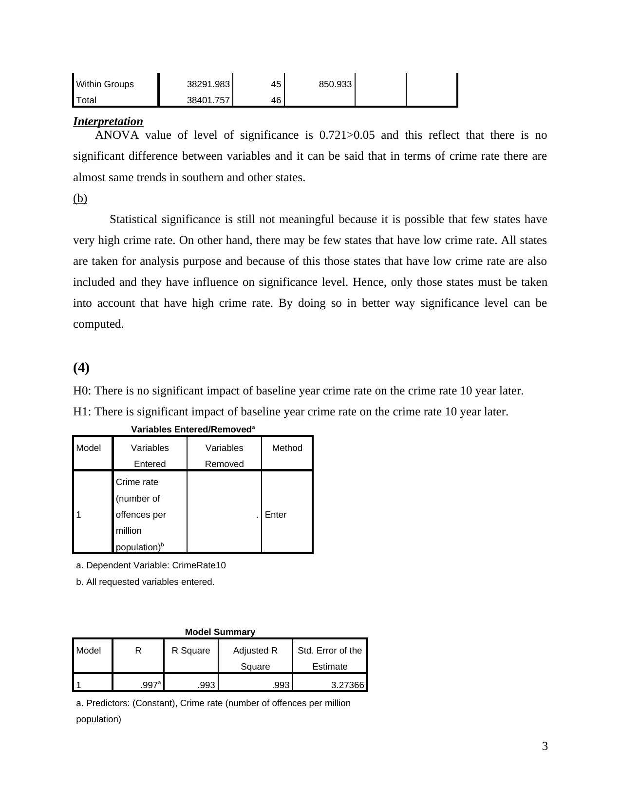
Within Groups 38291.983 45 850.933
Total 38401.757 46
Interpretation
ANOVA value of level of significance is 0.721>0.05 and this reflect that there is no
significant difference between variables and it can be said that in terms of crime rate there are
almost same trends in southern and other states.
(b)
Statistical significance is still not meaningful because it is possible that few states have
very high crime rate. On other hand, there may be few states that have low crime rate. All states
are taken for analysis purpose and because of this those states that have low crime rate are also
included and they have influence on significance level. Hence, only those states must be taken
into account that have high crime rate. By doing so in better way significance level can be
computed.
(4)
H0: There is no significant impact of baseline year crime rate on the crime rate 10 year later.
H1: There is significant impact of baseline year crime rate on the crime rate 10 year later.
Variables Entered/Removeda
Model Variables
Entered
Variables
Removed
Method
1
Crime rate
(number of
offences per
million
population)b
. Enter
a. Dependent Variable: CrimeRate10
b. All requested variables entered.
Model Summary
Model R R Square Adjusted R
Square
Std. Error of the
Estimate
1 .997a .993 .993 3.27366
a. Predictors: (Constant), Crime rate (number of offences per million
population)
3

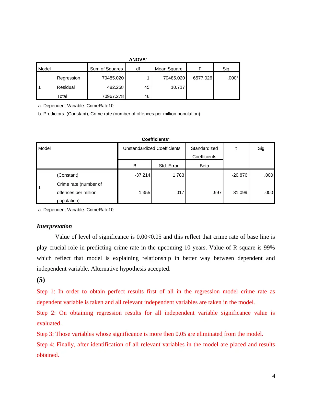
ANOVAa
Model Sum of Squares df Mean Square F Sig.
1
Regression 70485.020 1 70485.020 6577.026 .000b
Residual 482.258 45 10.717
Total 70967.278 46
a. Dependent Variable: CrimeRate10
b. Predictors: (Constant), Crime rate (number of offences per million population)
Coefficientsa
Model Unstandardized Coefficients Standardized
Coefficients
t Sig.
B Std. Error Beta
1
(Constant) -37.214 1.783 -20.876 .000
Crime rate (number of
offences per million
population)
1.355 .017 .997 81.099 .000
a. Dependent Variable: CrimeRate10
Interpretation
Value of level of significance is 0.00<0.05 and this reflect that crime rate of base line is
play crucial role in predicting crime rate in the upcoming 10 years. Value of R square is 99%
which reflect that model is explaining relationship in better way between dependent and
independent variable. Alternative hypothesis accepted.
(5)
Step 1: In order to obtain perfect results first of all in the regression model crime rate as
dependent variable is taken and all relevant independent variables are taken in the model.
Step 2: On obtaining regression results for all independent variable significance value is
evaluated.
Step 3: Those variables whose significance is more then 0.05 are eliminated from the model.
Step 4: Finally, after identification of all relevant variables in the model are placed and results
obtained.
4

Step 5: As per requirement again regression is run with same variable names but contain
performance of 10 year later. In this way entire calculation is done and given below.
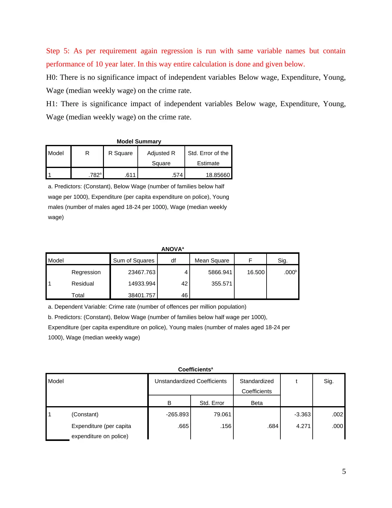
H0: There is no significance impact of independent variables Below wage, Expenditure, Young,
Wage (median weekly wage) on the crime rate.
H1: There is significance impact of independent variables Below wage, Expenditure, Young,
Wage (median weekly wage) on the crime rate.
Model Summary
Model R R Square Adjusted R
Square
Std. Error of the
Estimate
1 .782a .611 .574 18.85660
a. Predictors: (Constant), Below Wage (number of families below half
wage per 1000), Expenditure (per capita expenditure on police), Young
males (number of males aged 18-24 per 1000), Wage (median weekly
wage)
ANOVAa
Model Sum of Squares df Mean Square F Sig.
1
Regression 23467.763 4 5866.941 16.500 .000b
Residual 14933.994 42 355.571
Total 38401.757 46
a. Dependent Variable: Crime rate (number of offences per million population)
b. Predictors: (Constant), Below Wage (number of families below half wage per 1000),
Expenditure (per capita expenditure on police), Young males (number of males aged 18-24 per
1000), Wage (median weekly wage)
Coefficientsa
Model Unstandardized Coefficients Standardized
Coefficients
t Sig.
B Std. Error Beta
1 (Constant) -265.893 79.061 -3.363 .002
Expenditure (per capita
expenditure on police)
.665 .156 .684 4.271 .000
5

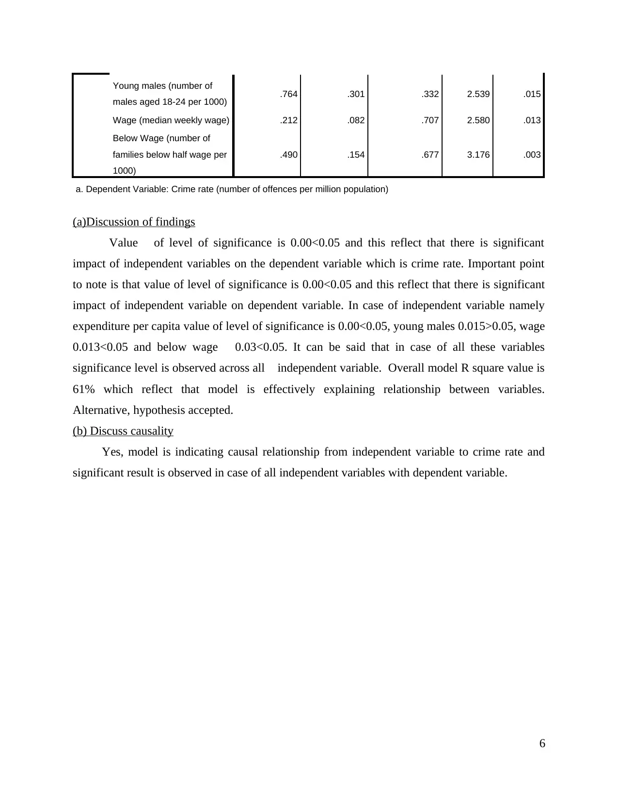
Young males (number of
males aged 18-24 per 1000) .764 .301 .332 2.539 .015
Wage (median weekly wage) .212 .082 .707 2.580 .013
Below Wage (number of
families below half wage per
1000)
.490 .154 .677 3.176 .003
a. Dependent Variable: Crime rate (number of offences per million population)
(a)Discussion of findings
Value of level of significance is 0.00<0.05 and this reflect that there is significant
impact of independent variables on the dependent variable which is crime rate. Important point
to note is that value of level of significance is 0.00<0.05 and this reflect that there is significant
impact of independent variable on dependent variable. In case of independent variable namely
expenditure per capita value of level of significance is 0.00<0.05, young males 0.015>0.05, wage
0.013<0.05 and below wage 0.03<0.05. It can be said that in case of all these variables
significance level is observed across all independent variable. Overall model R square value is
61% which reflect that model is effectively explaining relationship between variables.
Alternative, hypothesis accepted.
(b) Discuss causality
Yes, model is indicating causal relationship from independent variable to crime rate and
significant result is observed in case of all independent variables with dependent variable.
6

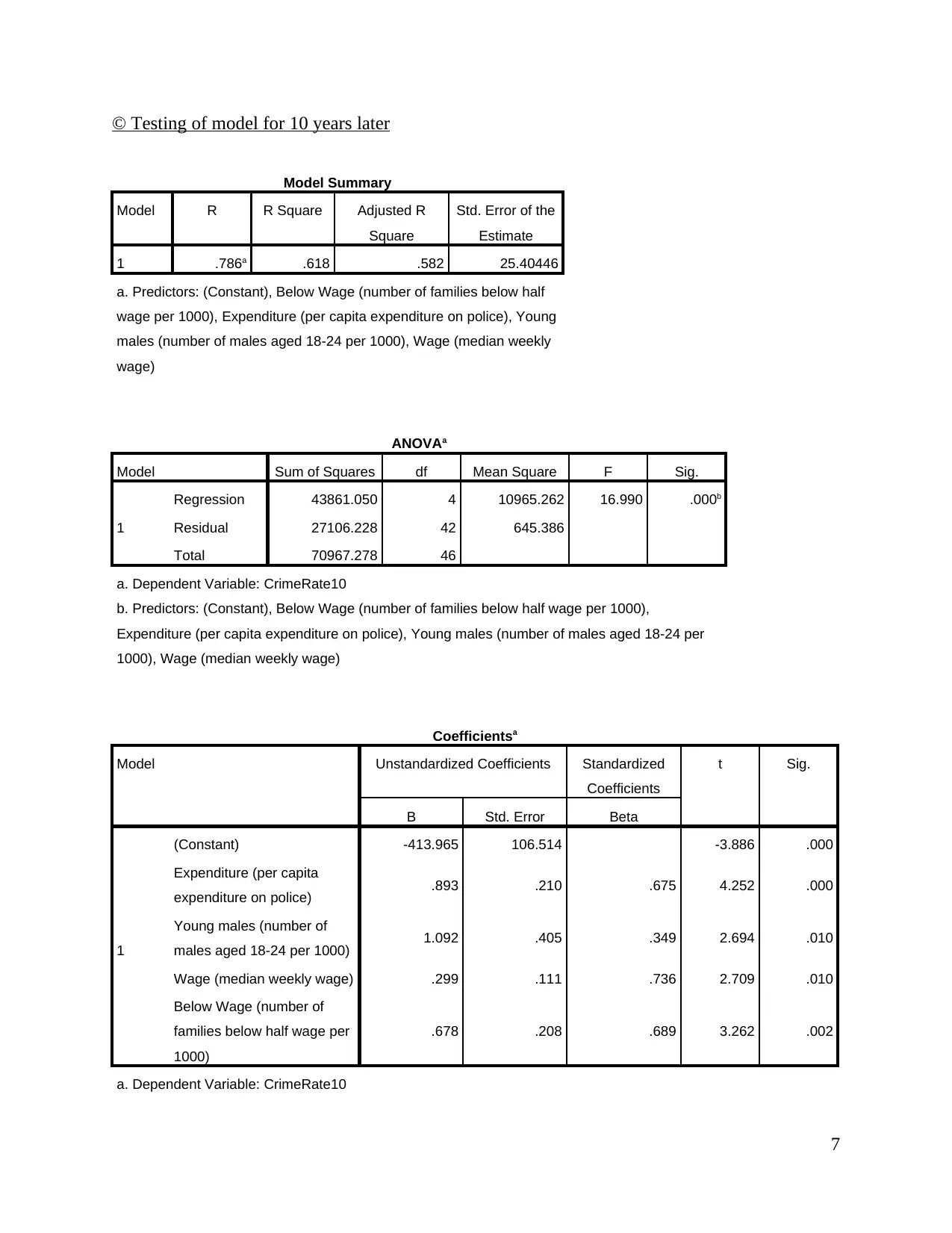
© Testing of model for 10 years later
Model Summary
Model R R Square Adjusted R
Square
Std. Error of the
Estimate
1 .786a .618 .582 25.40446
a. Predictors: (Constant), Below Wage (number of families below half
wage per 1000), Expenditure (per capita expenditure on police), Young
males (number of males aged 18-24 per 1000), Wage (median weekly
wage)
ANOVAa
Model Sum of Squares df Mean Square F Sig.
1
Regression 43861.050 4 10965.262 16.990 .000b
Residual 27106.228 42 645.386
Total 70967.278 46
a. Dependent Variable: CrimeRate10
b. Predictors: (Constant), Below Wage (number of families below half wage per 1000),
Expenditure (per capita expenditure on police), Young males (number of males aged 18-24 per
1000), Wage (median weekly wage)
Coefficientsa
Model Unstandardized Coefficients Standardized
Coefficients
t Sig.
B Std. Error Beta
1
(Constant) -413.965 106.514 -3.886 .000
Expenditure (per capita
expenditure on police) .893 .210 .675 4.252 .000
Young males (number of
males aged 18-24 per 1000) 1.092 .405 .349 2.694 .010
Wage (median weekly wage) .299 .111 .736 2.709 .010
Below Wage (number of
families below half wage per
1000)
.678 .208 .689 3.262 .002
a. Dependent Variable: CrimeRate10
7

Model is equally successful and there is slight difference in the significance level. In case of
independent variable namely expenditure per capita value of level of significance is 0.00<0.05
for baseline year and same for 10 year later, young males 0.015>0.05 for baseline year and
0.010<0.05 for 10 year later, wage 0.013<0.05 and 0.10>0.05 for 10 year later and below wage
0.03<0.05 and 0.002<0.05 for 10 year later. It can be said that almost similar results are obtained
on re run of model. In case of variable crime rate 10 year also significance is observed. Hence,
alternative hypothesis accepted.
(6)
Group Statistics
Class N Mean Std. Deviation Std. Error Mean
Age 1st 284 39.16 14.548 .863
2nd 261 29.51 13.639 .844
Independent Samples Test
Levene's Test for
Equality of
Variances
t-test for Equality of Means
F Sig. t df Sig. (2-
tailed)
Mean
Difference
Std. Error
Difference
95% Confidence
Interval of the
Difference
Lower Upper
Age
Equal variances
assumed 5.894 .016 7.973 543 .000 9.653 1.211 7.275 12.032
Equal variances
not assumed 7.995 542.782 .000 9.653 1.207 7.281 12.025
Group Statistics
Class N Mean Std. Deviation Std. Error Mean
Age 2nd 261 29.51 13.639 .844
3rd 501 24.82 11.958 .534
8

Independent Samples Test
Levene's Test for
Equality of
Variances
t-test for Equality of Means
F Sig. t df Sig. (2-
tailed)
Mean
Difference
Std. Error
Difference
95% Confidence
Interval of the
Difference
Lower Upper
Age
Equal variances
assumed 4.107 .043 4.893 760 .000 4.690 .959 2.808 6.572
Equal variances
not assumed 4.695 470.699 .000 4.690 .999 2.727 6.654
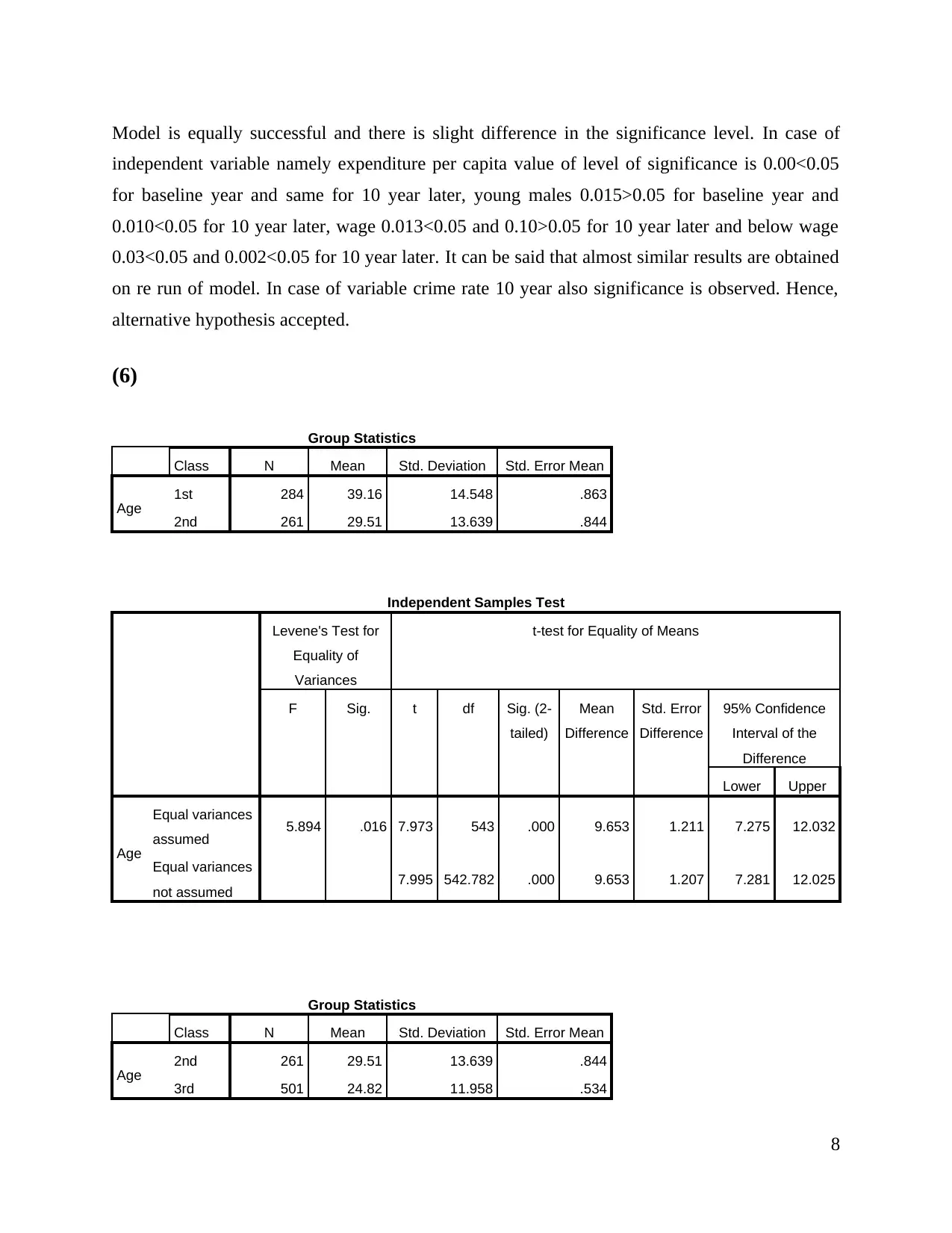
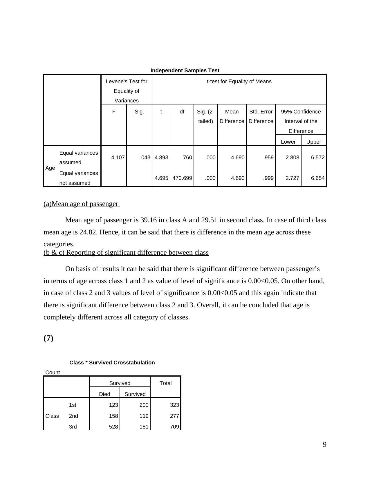
(a)Mean age of passenger
Mean age of passenger is 39.16 in class A and 29.51 in second class. In case of third class
mean age is 24.82. Hence, it can be said that there is difference in the mean age across these
categories.
(b & c) Reporting of significant difference between class
On basis of results it can be said that there is significant difference between passenger’s
in terms of age across class 1 and 2 as value of level of significance is 0.00<0.05. On other hand,
in case of class 2 and 3 values of level of significance is 0.00<0.05 and this again indicate that
there is significant difference between class 2 and 3. Overall, it can be concluded that age is
completely different across all category of classes.
(7)
Class * Survived Crosstabulation
Count
Survived Total
Died Survived
Class
1st 123 200 323
2nd 158 119 277
3rd 528 181 709
9

Total 809 500 1309
Chi-Square Tests
Value df Asymp. Sig. (2-
sided)
Pearson Chi-Square 127.859a 2 .000
Likelihood Ratio 127.765 2 .000
Linear-by-Linear Association 127.709 1 .000
N of Valid Cases 1309
a. 0 cells (0.0%) have expected count less than 5. The minimum
expected count is 105.81.
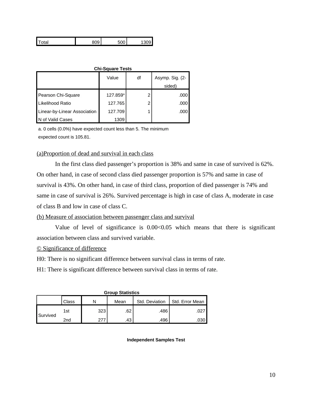
(a)Proportion of dead and survival in each class
In the first class died passenger’s proportion is 38% and same in case of survived is 62%.
On other hand, in case of second class died passenger proportion is 57% and same in case of
survival is 43%. On other hand, in case of third class, proportion of died passenger is 74% and
same in case of survival is 26%. Survived percentage is high in case of class A, moderate in case
of class B and low in case of class C.
(b) Measure of association between passenger class and survival
Value of level of significance is 0.00<0.05 which means that there is significant
association between class and survived variable.
© Significance of difference
H0: There is no significant difference between survival class in terms of rate.
H1: There is significant difference between survival class in terms of rate.
Group Statistics
Class N Mean Std. Deviation Std. Error Mean
Survived 1st 323 .62 .486 .027
2nd 277 .43 .496 .030
Independent Samples Test
10

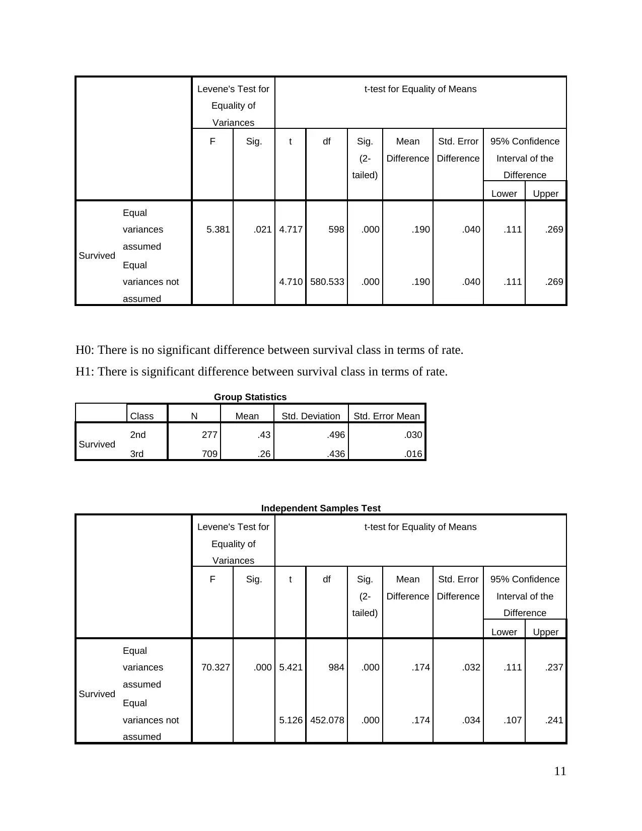
Levene's Test for
Equality of
Variances
t-test for Equality of Means
F Sig. t df Sig.
(2-
tailed)
Mean
Difference
Std. Error
Difference
95% Confidence
Interval of the
Difference
Lower Upper
Survived
Equal
variances
assumed
5.381 .021 4.717 598 .000 .190 .040 .111 .269
Equal
variances not
assumed
4.710 580.533 .000 .190 .040 .111 .269
H0: There is no significant difference between survival class in terms of rate.
H1: There is significant difference between survival class in terms of rate.
Group Statistics
Class N Mean Std. Deviation Std. Error Mean
Survived 2nd 277 .43 .496 .030
3rd 709 .26 .436 .016
Independent Samples Test
Levene's Test for
Equality of
Variances
t-test for Equality of Means
F Sig. t df Sig.
(2-
tailed)
Mean
Difference
Std. Error
Difference
95% Confidence
Interval of the
Difference
Lower Upper
Survived
Equal
variances
assumed
70.327 .000 5.421 984 .000 .174 .032 .111 .237
Equal
variances not
assumed
5.126 452.078 .000 .174 .034 .107 .241
11

Value of level of significance is 0.00<0.05 in case of both models and it can be said that there is
significant difference between class and survival rate. Alternative, hypothesis accepted in case of
both models.
12

REFERENCES
Books and Journals
Camilleri, S.F., 2017. Theory, probability, and induction in social research. In Sociological
Methods (pp. 70-83). Routledge.
Williams, R. and Bornmann, L., 2016. Sampling issues in bibliometric analysis. Journal of
Informetrics. 10(4). pp.1225-1232.
Online
Sampling distribution definition, types and classes., 2019. [Online]. Available through:<
https://www.statisticshowto.datasciencecentral.com/sampling-distribution/>.
13