Bank Branch Waiting Time Analysis

This assignment analyzes the waiting time at two different bank branches: Perth CBD and Suburban. It requires performing a hypothesis test to determine if there is a significant difference in their variances and mean waiting times. The analysis uses t-tests with PhStat software, presenting hypothesis testing steps, tables of results, and a conclusion summarizing the findings.

Quantitative skills for business
Name
University
9th October 2017

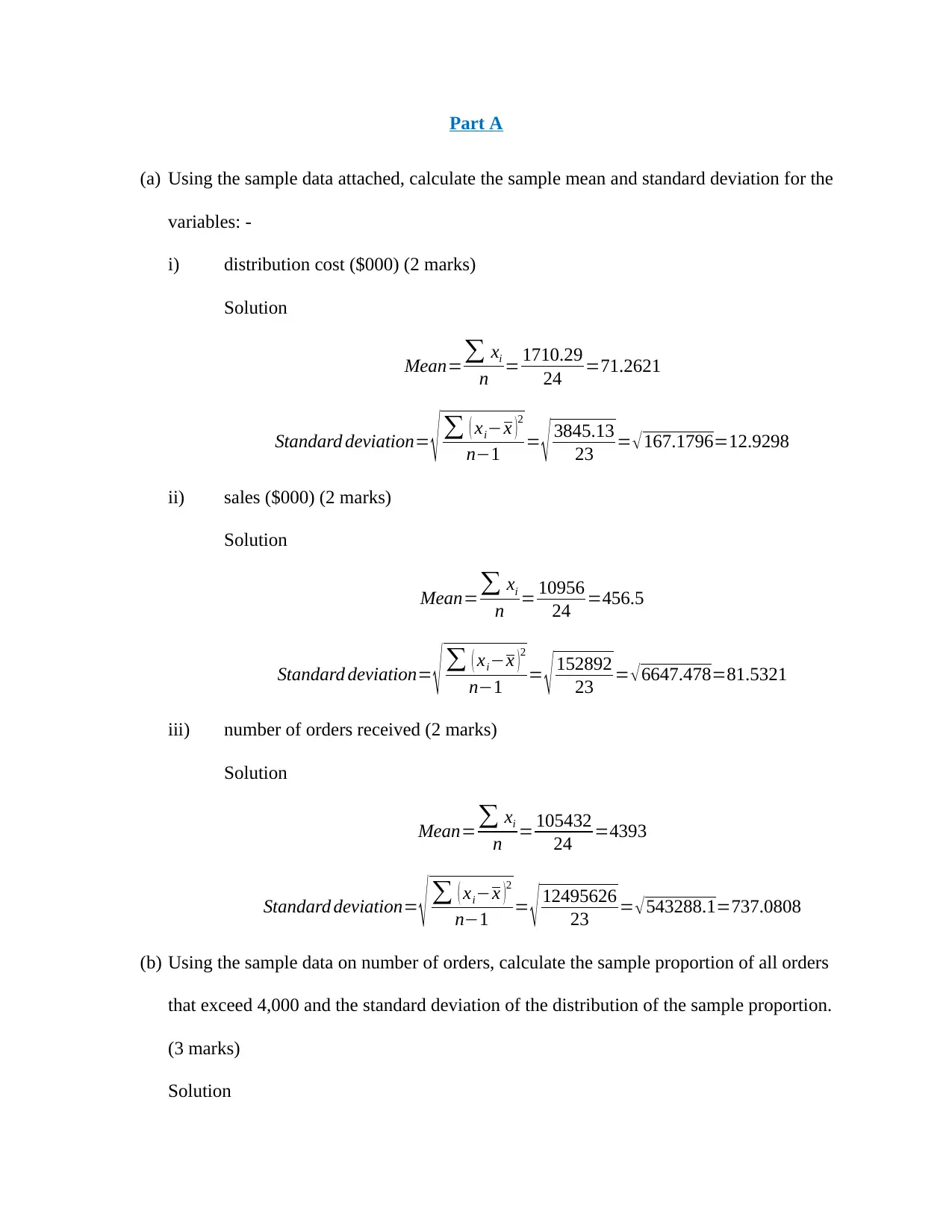
Part A
(a) Using the sample data attached, calculate the sample mean and standard deviation for the
variables: -
i) distribution cost ($000) (2 marks)
Solution
Mean=∑ xi
n = 1710.29
24 =71.2621
Standard deviation= √ ∑ ( xi−x )2
n−1 = √ 3845.13
23 = √167.1796=12.9298
ii) sales ($000) (2 marks)
Solution
Mean=∑ xi
n = 10956
24 =456.5
Standard deviation= √ ∑ ( xi−x )2
n−1 = √ 152892
23 = √6647.478=81.5321
iii) number of orders received (2 marks)
Solution
Mean=∑ xi
n = 105432
24 =4393
Standard deviation= √ ∑ ( xi−x )2
n−1 = √ 12495626
23 = √543288.1=737.0808
(b) Using the sample data on number of orders, calculate the sample proportion of all orders
that exceed 4,000 and the standard deviation of the distribution of the sample proportion.
(3 marks)
Solution

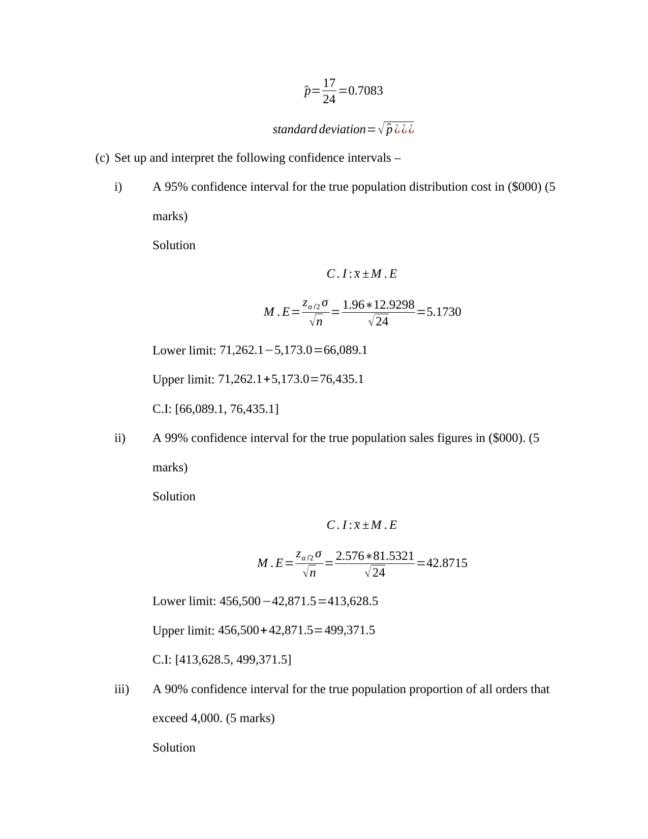
^p= 17
24 =0.7083
standard deviation= √ ^p ¿ ¿ ¿
(c) Set up and interpret the following confidence intervals –
i) A 95% confidence interval for the true population distribution cost in ($000) (5
marks)
Solution
C . I : x ± M . E
M . E= zα /2 σ
√n = 1.96∗12.9298
√24 =5.1730
Lower limit: 71,262.1−5,173.0=66,089.1
Upper limit: 71,262.1+5,173.0=76,435.1
C.I: [66,089.1, 76,435.1]
ii) A 99% confidence interval for the true population sales figures in ($000). (5
marks)
Solution
C . I : x ± M . E
M . E= zα /2 σ
√ n = 2.576∗81.5321
√ 24 =42.8715
Lower limit: 456,500−42,871.5=413,628.5
Upper limit: 456,500+ 42,871.5=499,371.5
C.I: [413,628.5, 499,371.5]
iii) A 90% confidence interval for the true population proportion of all orders that
exceed 4,000. (5 marks)
Solution

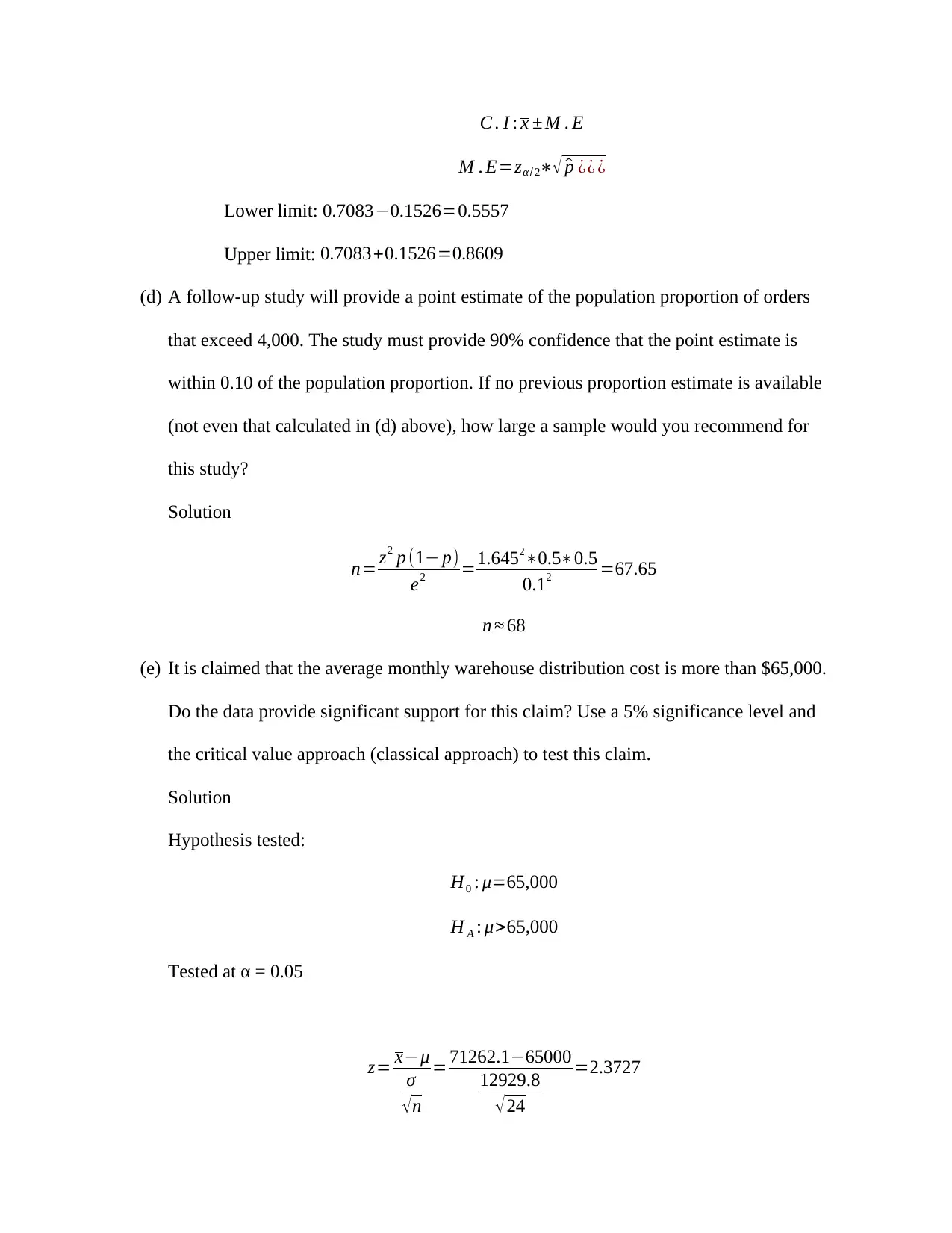
C . I : x ± M . E
M . E=zα / 2∗√ ^p ¿¿ ¿
Lower limit: 0.7083−0.1526=0.5557
Upper limit: 0.7083+0.1526=0.8609
(d) A follow-up study will provide a point estimate of the population proportion of orders
that exceed 4,000. The study must provide 90% confidence that the point estimate is
within 0.10 of the population proportion. If no previous proportion estimate is available
(not even that calculated in (d) above), how large a sample would you recommend for
this study?
Solution
n= z2 p (1− p)
e2 =1.6452∗0.5∗0.5
0.12 =67.65
n ≈ 68
(e) It is claimed that the average monthly warehouse distribution cost is more than $65,000.
Do the data provide significant support for this claim? Use a 5% significance level and
the critical value approach (classical approach) to test this claim.
Solution
Hypothesis tested:
H0 : μ=65,000
H A : μ>65,000
Tested at α = 0.05
z= x−μ
σ
√ n
= 71262.1−65000
12929.8
√ 24
=2.3727

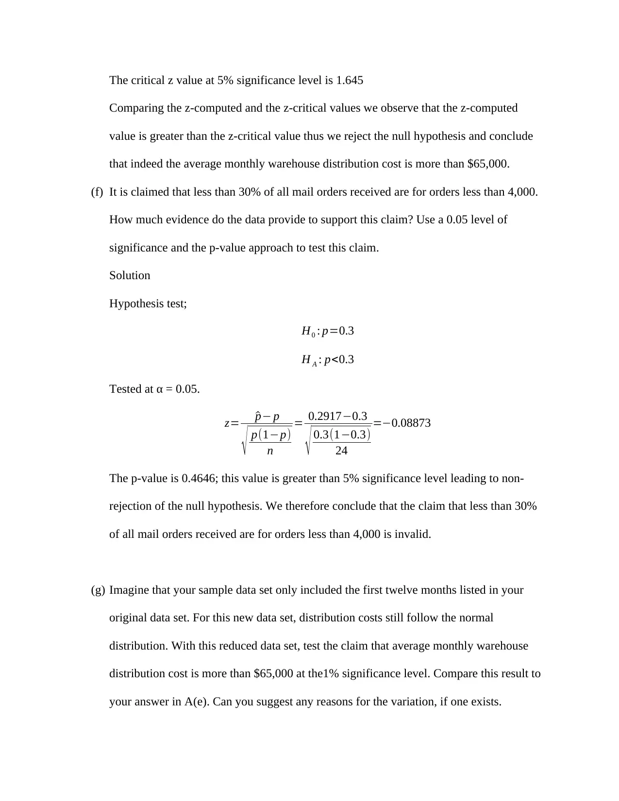
The critical z value at 5% significance level is 1.645
Comparing the z-computed and the z-critical values we observe that the z-computed
value is greater than the z-critical value thus we reject the null hypothesis and conclude
that indeed the average monthly warehouse distribution cost is more than $65,000.
(f) It is claimed that less than 30% of all mail orders received are for orders less than 4,000.
How much evidence do the data provide to support this claim? Use a 0.05 level of
significance and the p-value approach to test this claim.
Solution
Hypothesis test;
H0 : p=0.3
H A : p<0.3
Tested at α = 0.05.
z= ^p− p
√ p(1−p)
n
= 0.2917−0.3
√ 0.3(1−0.3)
24
=−0.08873
The p-value is 0.4646; this value is greater than 5% significance level leading to non-
rejection of the null hypothesis. We therefore conclude that the claim that less than 30%
of all mail orders received are for orders less than 4,000 is invalid.
(g) Imagine that your sample data set only included the first twelve months listed in your
original data set. For this new data set, distribution costs still follow the normal
distribution. With this reduced data set, test the claim that average monthly warehouse
distribution cost is more than $65,000 at the1% significance level. Compare this result to
your answer in A(e). Can you suggest any reasons for the variation, if one exists.

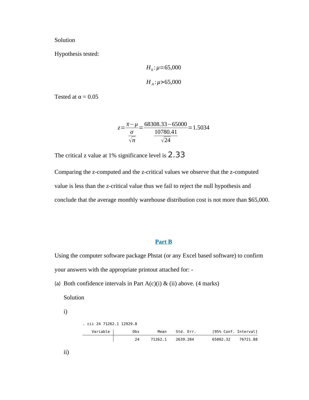
Solution
Hypothesis tested:
H0 : μ=65,000
H A : μ>65,000
Tested at α = 0.05
z= x−μ
σ
√ n
= 68308.33−65000
10780.41
√ 24
=1.5034
The critical z value at 1% significance level is 2.33
Comparing the z-computed and the z-critical values we observe that the z-computed
value is less than the z-critical value thus we fail to reject the null hypothesis and
conclude that the average monthly warehouse distribution cost is not more than $65,000.
Part B
Using the computer software package Phstat (or any Excel based software) to confirm
your answers with the appropriate printout attached for: -
(a) Both confidence intervals in Part A(c)(i) & (ii) above. (4 marks)
Solution
i)
24 71262.1 2639.284 65802.32 76721.88
Variable Obs Mean Std. Err. [95% Conf. Interval]
. cii 24 71262.1 12929.8
ii)

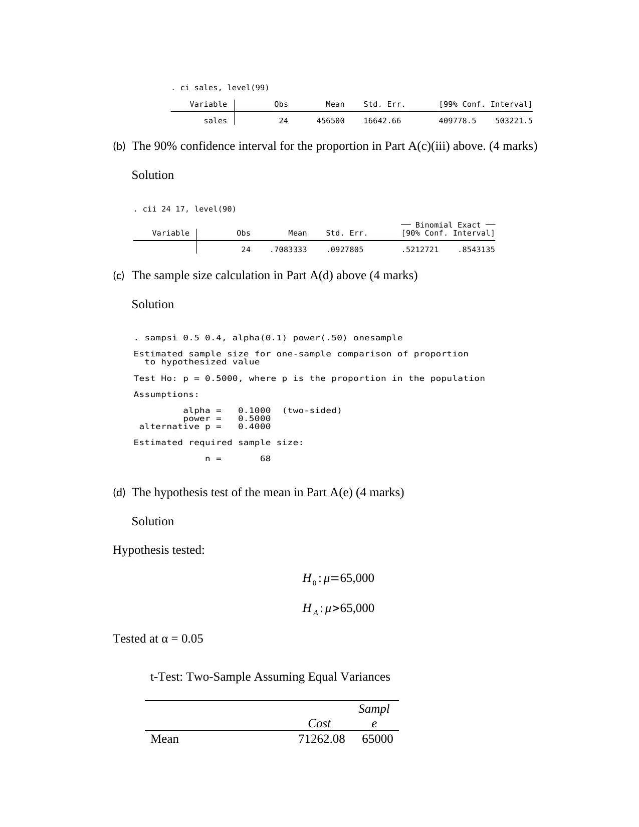
sales 24 456500 16642.66 409778.5 503221.5
Variable Obs Mean Std. Err. [99% Conf. Interval]
. ci sales, level(99)
(b) The 90% confidence interval for the proportion in Part A(c)(iii) above. (4 marks)
Solution
24 .7083333 .0927805 .5212721 .8543135
Variable Obs Mean Std. Err. [90% Conf. Interval]
Binomial Exact
. cii 24 17, level(90)
(c) The sample size calculation in Part A(d) above (4 marks)
Solution
n = 68
Estimated required sample size:
alternative p = 0.4000
power = 0.5000
alpha = 0.1000 (two-sided)
Assumptions:
Test Ho: p = 0.5000, where p is the proportion in the population
to hypothesized value
Estimated sample size for one-sample comparison of proportion
. sampsi 0.5 0.4, alpha(0.1) power(.50) onesample
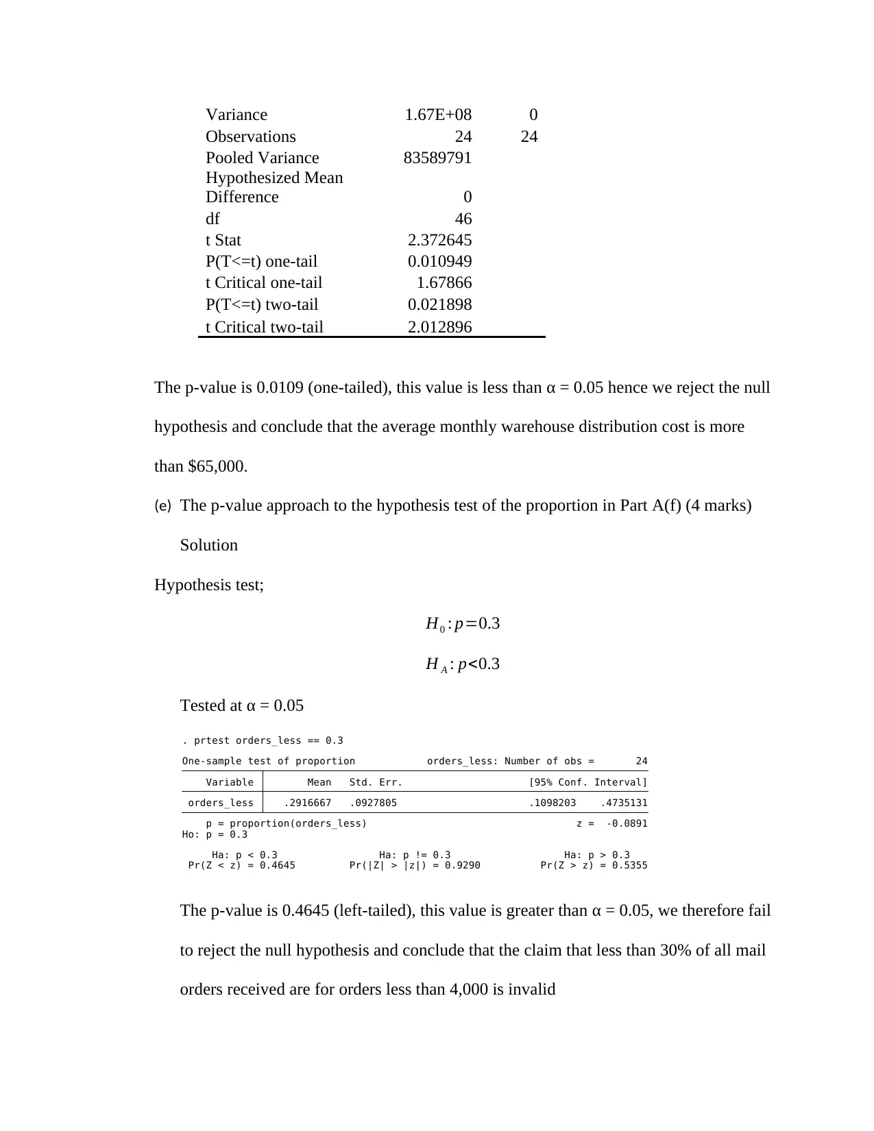
(d) The hypothesis test of the mean in Part A(e) (4 marks)
Solution
Hypothesis tested:
H0 : μ=65,000
H A : μ>65,000
Tested at α = 0.05
t-Test: Two-Sample Assuming Equal Variances
Cost
Sampl
e
Mean 71262.08 65000

Variance 1.67E+08 0
Observations 24 24
Pooled Variance 83589791
Hypothesized Mean
Difference 0
df 46
t Stat 2.372645
P(T<=t) one-tail 0.010949
t Critical one-tail 1.67866
P(T<=t) two-tail 0.021898
t Critical two-tail 2.012896
The p-value is 0.0109 (one-tailed), this value is less than α = 0.05 hence we reject the null
hypothesis and conclude that the average monthly warehouse distribution cost is more
than $65,000.
(e) The p-value approach to the hypothesis test of the proportion in Part A(f) (4 marks)
Solution
Hypothesis test;
H0 : p=0.3
H A : p<0.3
Tested at α = 0.05
Pr(Z < z) = 0.4645 Pr(|Z| > |z|) = 0.9290 Pr(Z > z) = 0.5355
Ha: p < 0.3 Ha: p != 0.3 Ha: p > 0.3
Ho: p = 0.3
p = proportion(orders_less) z = -0.0891
orders_less .2916667 .0927805 .1098203 .4735131
Variable Mean Std. Err. [95% Conf. Interval]
One-sample test of proportion orders_less: Number of obs = 24
. prtest orders_less == 0.3
The p-value is 0.4645 (left-tailed), this value is greater than α = 0.05, we therefore fail
to reject the null hypothesis and conclude that the claim that less than 30% of all mail
orders received are for orders less than 4,000 is invalid

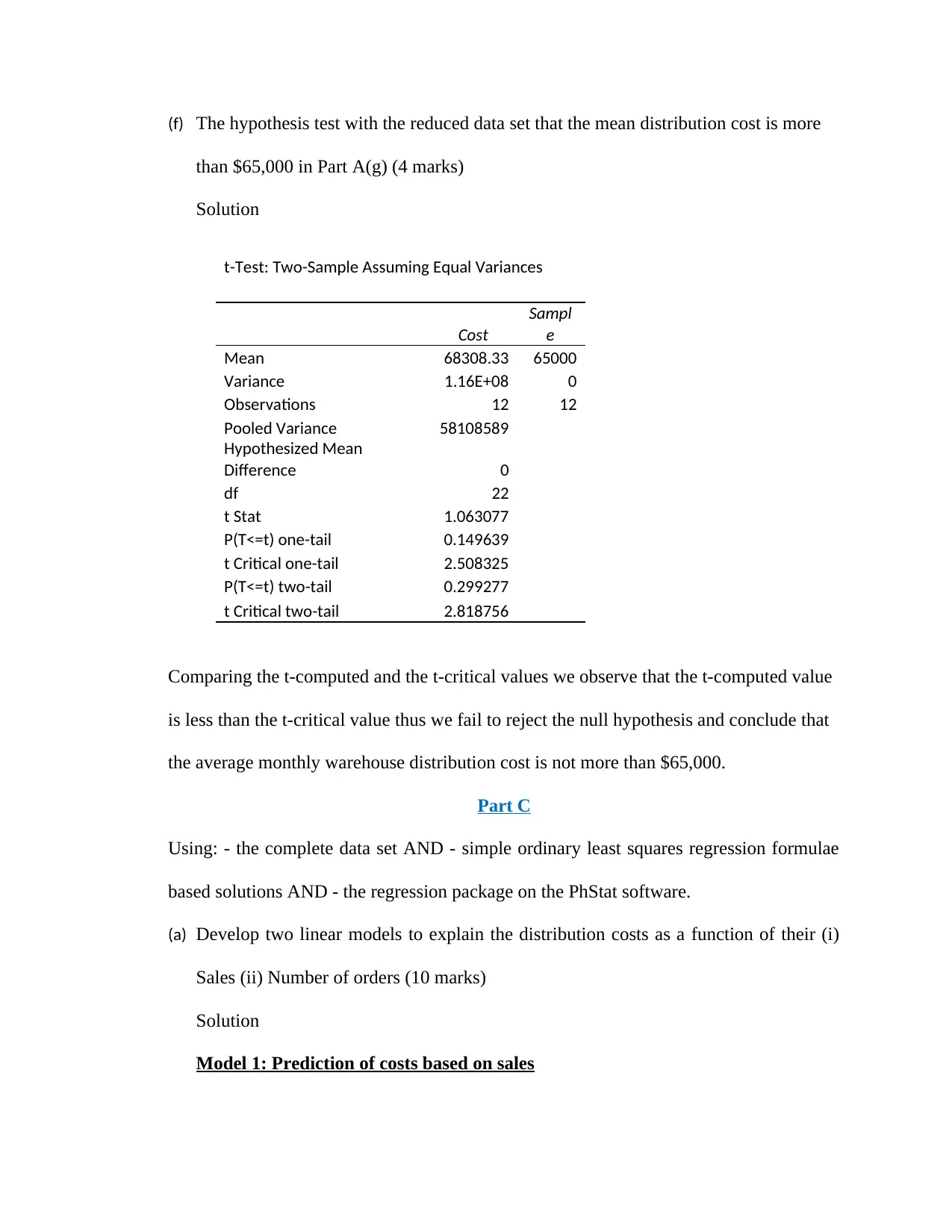
(f) The hypothesis test with the reduced data set that the mean distribution cost is more
than $65,000 in Part A(g) (4 marks)
Solution
t-Test: Two-Sample Assuming Equal Variances
Cost
Sampl
e
Mean 68308.33 65000
Variance 1.16E+08 0
Observations 12 12
Pooled Variance 58108589
Hypothesized Mean
Difference 0
df 22
t Stat 1.063077
P(T<=t) one-tail 0.149639
t Critical one-tail 2.508325
P(T<=t) two-tail 0.299277
t Critical two-tail 2.818756
Comparing the t-computed and the t-critical values we observe that the t-computed value
is less than the t-critical value thus we fail to reject the null hypothesis and conclude that
the average monthly warehouse distribution cost is not more than $65,000.
Part C
Using: - the complete data set AND - simple ordinary least squares regression formulae
based solutions AND - the regression package on the PhStat software.
(a) Develop two linear models to explain the distribution costs as a function of their (i)
Sales (ii) Number of orders (10 marks)
Solution
Model 1: Prediction of costs based on sales

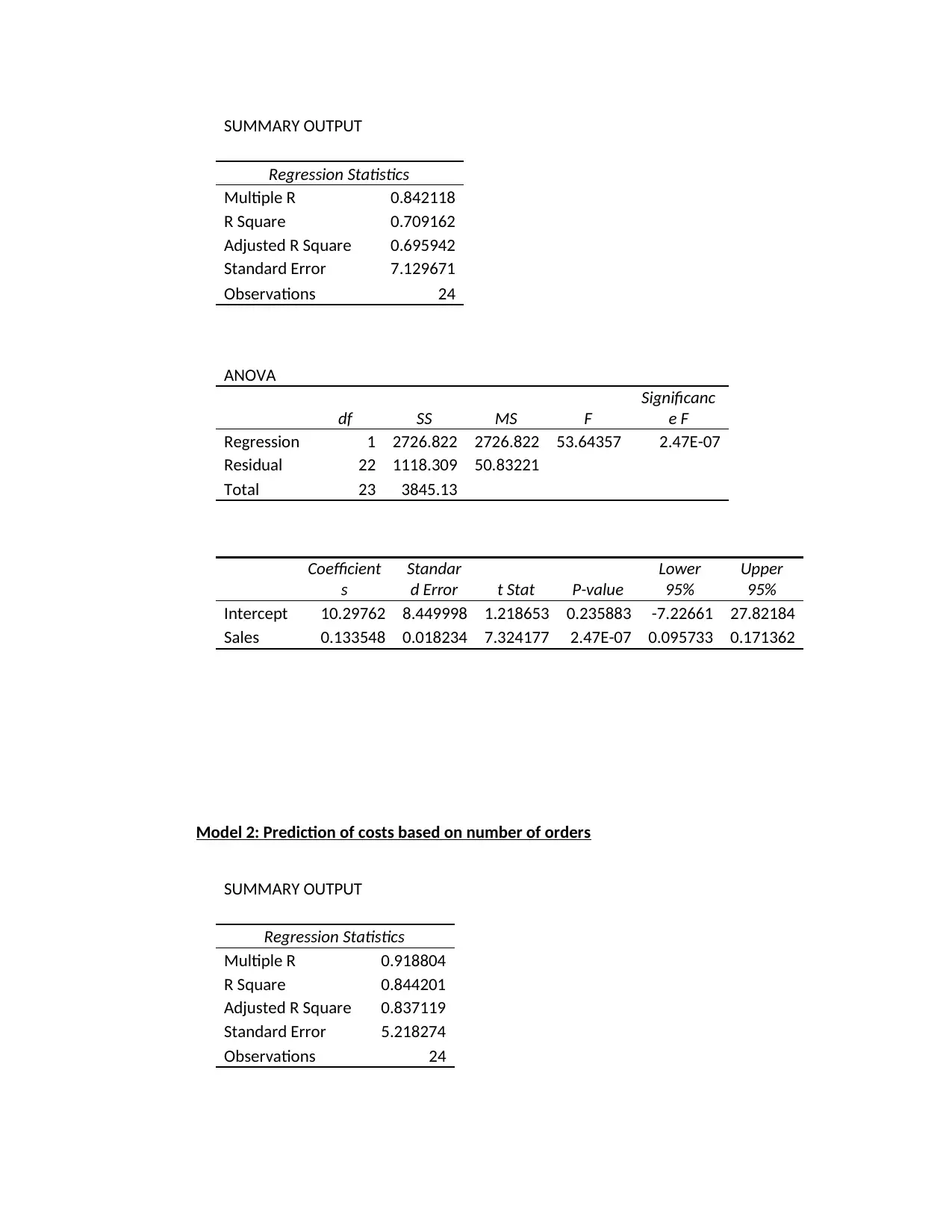
SUMMARY OUTPUT
Regression Statistics
Multiple R 0.842118
R Square 0.709162
Adjusted R Square 0.695942
Standard Error 7.129671
Observations 24
ANOVA
df SS MS F
Significanc
e F
Regression 1 2726.822 2726.822 53.64357 2.47E-07
Residual 22 1118.309 50.83221
Total 23 3845.13
Coefficient
s
Standar
d Error t Stat P-value
Lower
95%
Upper
95%
Intercept 10.29762 8.449998 1.218653 0.235883 -7.22661 27.82184
Sales 0.133548 0.018234 7.324177 2.47E-07 0.095733 0.171362
Model 2: Prediction of costs based on number of orders
SUMMARY OUTPUT
Regression Statistics
Multiple R 0.918804
R Square 0.844201
Adjusted R Square 0.837119
Standard Error 5.218274
Observations 24

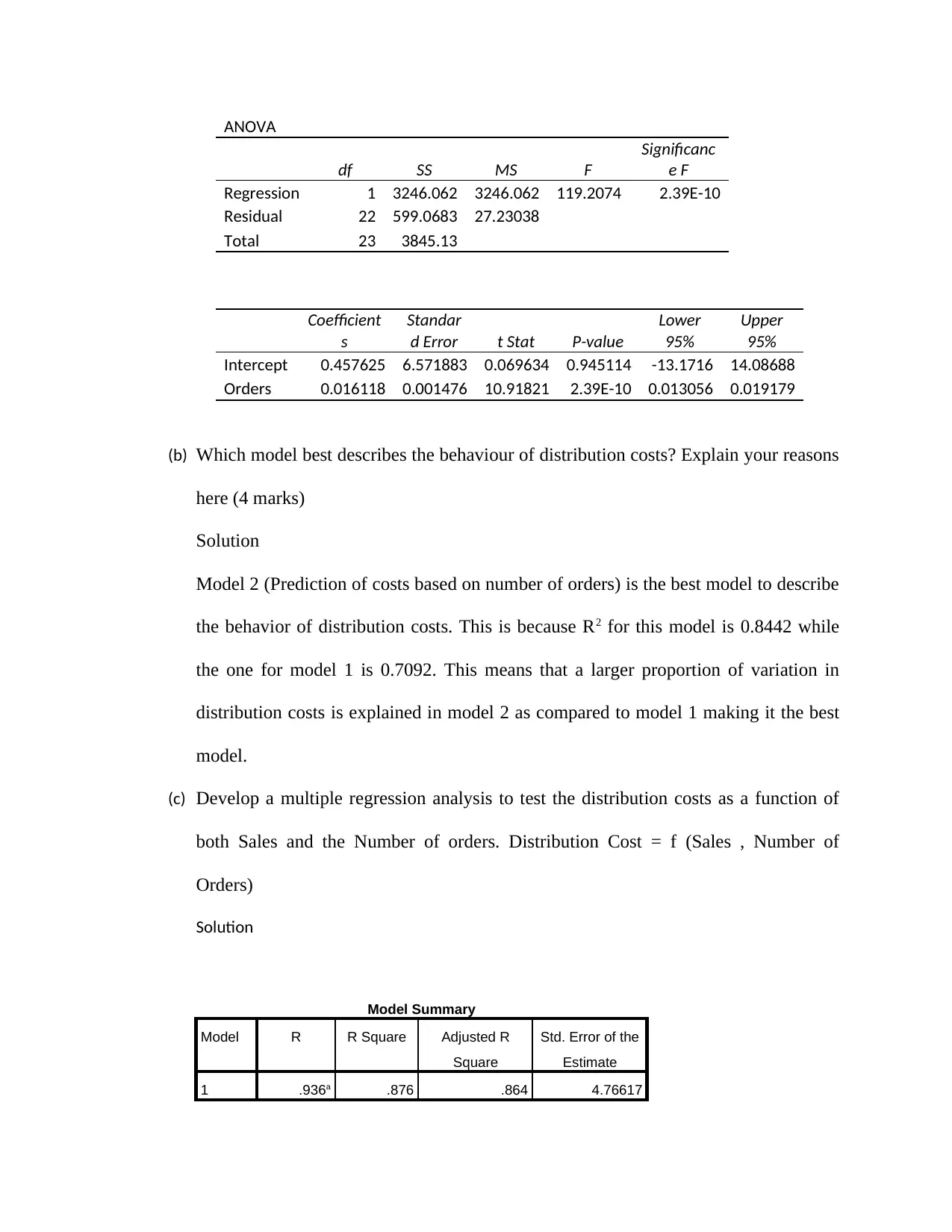
ANOVA
df SS MS F
Significanc
e F
Regression 1 3246.062 3246.062 119.2074 2.39E-10
Residual 22 599.0683 27.23038
Total 23 3845.13
Coefficient
s
Standar
d Error t Stat P-value
Lower
95%
Upper
95%
Intercept 0.457625 6.571883 0.069634 0.945114 -13.1716 14.08688
Orders 0.016118 0.001476 10.91821 2.39E-10 0.013056 0.019179
(b) Which model best describes the behaviour of distribution costs? Explain your reasons
here (4 marks)
Solution
Model 2 (Prediction of costs based on number of orders) is the best model to describe
the behavior of distribution costs. This is because R2 for this model is 0.8442 while
the one for model 1 is 0.7092. This means that a larger proportion of variation in
distribution costs is explained in model 2 as compared to model 1 making it the best
model.
(c) Develop a multiple regression analysis to test the distribution costs as a function of
both Sales and the Number of orders. Distribution Cost = f (Sales , Number of
Orders)
Solution
Model Summary
Model R R Square Adjusted R
Square
Std. Error of the
Estimate
1 .936a .876 .864 4.76617

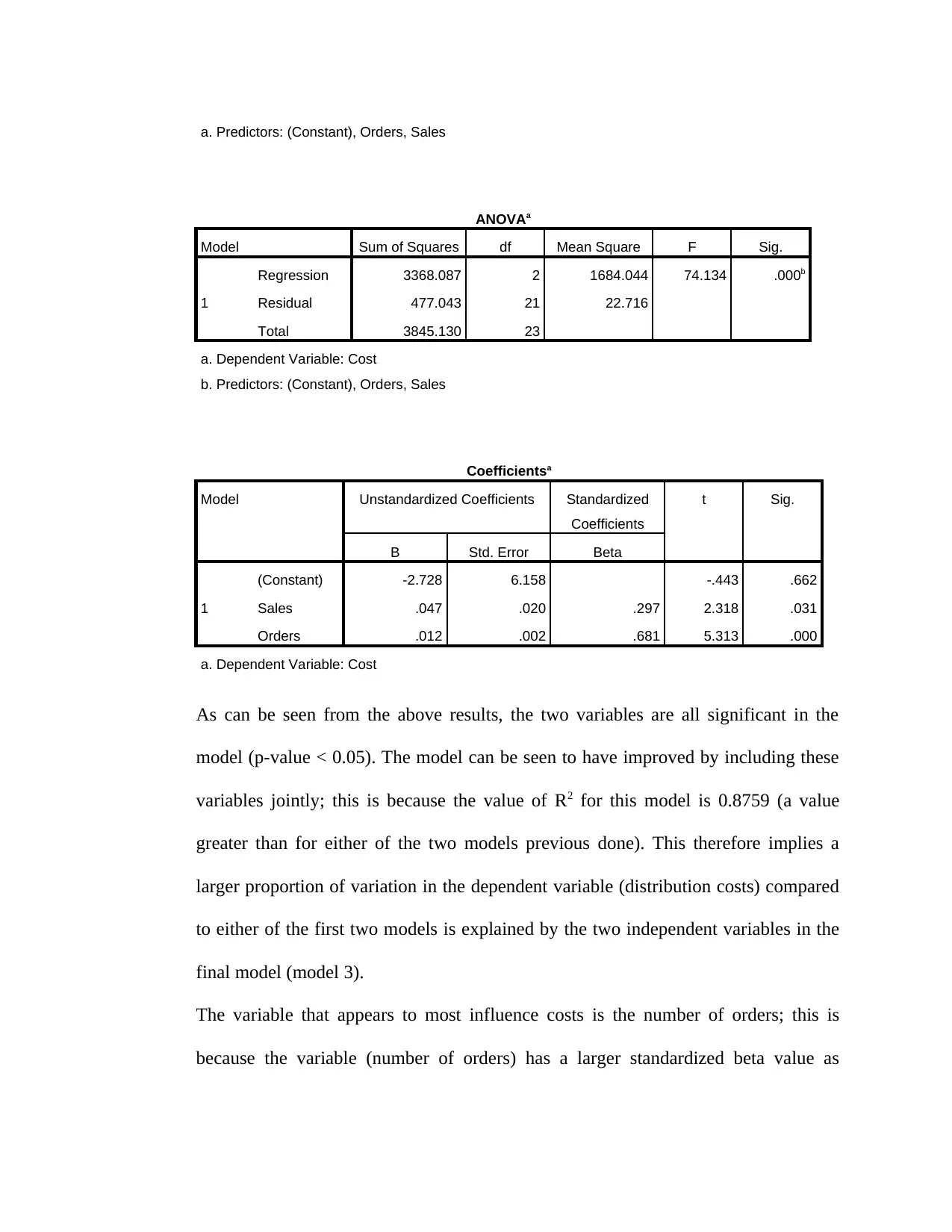
a. Predictors: (Constant), Orders, Sales
ANOVAa
Model Sum of Squares df Mean Square F Sig.
1
Regression 3368.087 2 1684.044 74.134 .000b
Residual 477.043 21 22.716
Total 3845.130 23
a. Dependent Variable: Cost
b. Predictors: (Constant), Orders, Sales
Coefficientsa
Model Unstandardized Coefficients Standardized
Coefficients
t Sig.
B Std. Error Beta
1
(Constant) -2.728 6.158 -.443 .662
Sales .047 .020 .297 2.318 .031
Orders .012 .002 .681 5.313 .000
a. Dependent Variable: Cost
As can be seen from the above results, the two variables are all significant in the
model (p-value < 0.05). The model can be seen to have improved by including these
variables jointly; this is because the value of R2 for this model is 0.8759 (a value
greater than for either of the two models previous done). This therefore implies a
larger proportion of variation in the dependent variable (distribution costs) compared
to either of the first two models is explained by the two independent variables in the
final model (model 3).
The variable that appears to most influence costs is the number of orders; this is
because the variable (number of orders) has a larger standardized beta value as

compared to the other variable (sales). This implies that it (orders) has more influence
on the dependent variable (distribution costs) as compared to the sales.
The final regression equation model is given as follows
Distribution Cost=−2.7283+0.0471 ( Sales ) +0.0119(Orders)
Part D
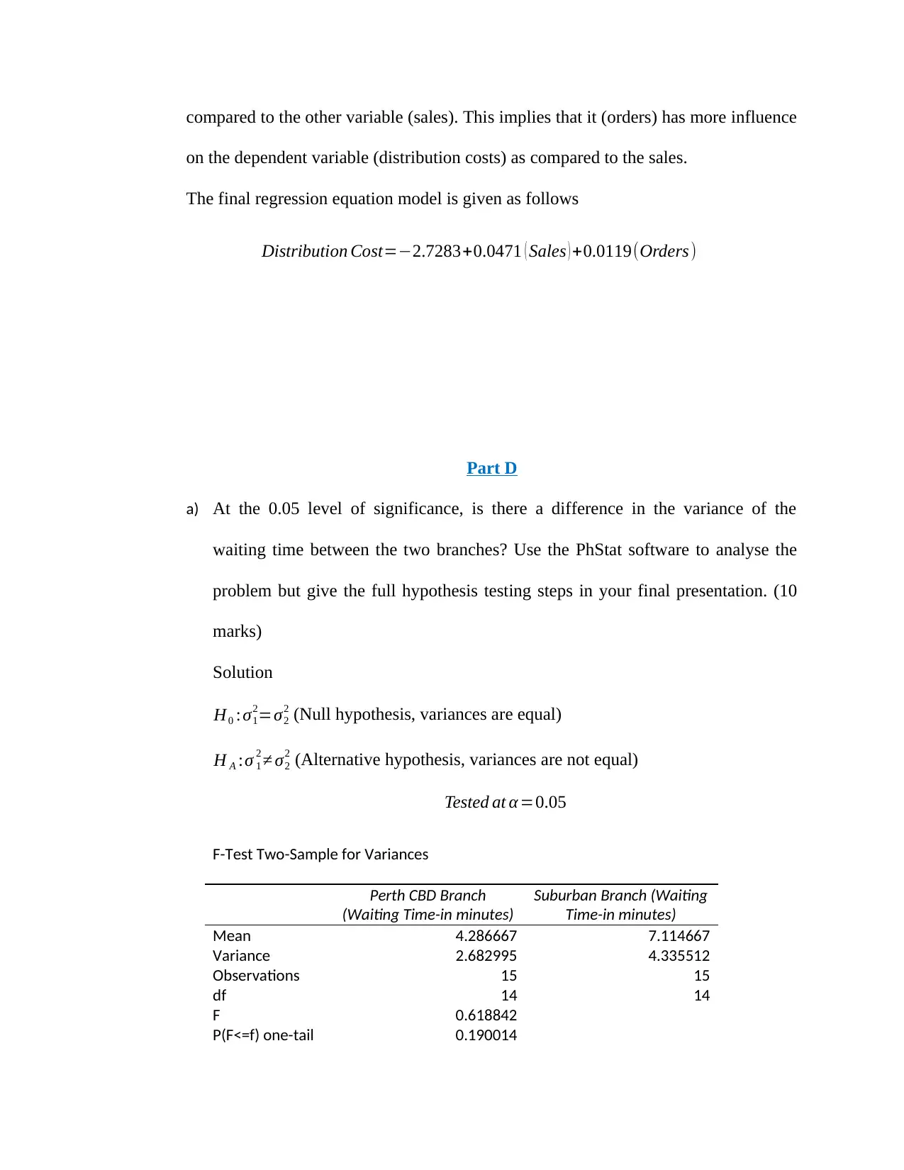
a) At the 0.05 level of significance, is there a difference in the variance of the
waiting time between the two branches? Use the PhStat software to analyse the
problem but give the full hypothesis testing steps in your final presentation. (10
marks)
Solution
H0 :σ1
2=σ2
2 (Null hypothesis, variances are equal)
H A :σ 1
2 ≠ σ2
2 (Alternative hypothesis, variances are not equal)
Tested at α =0.05
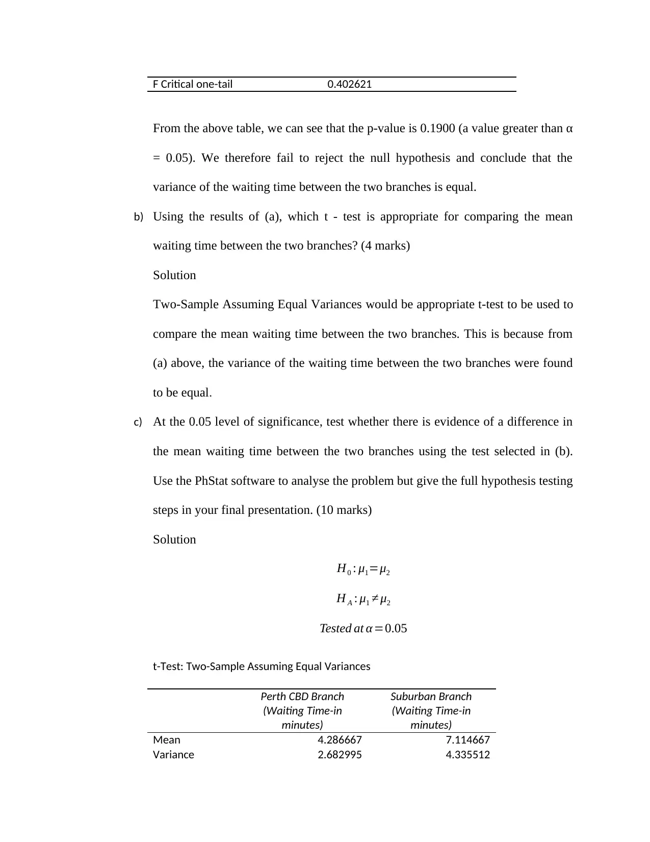
F-Test Two-Sample for Variances
Perth CBD Branch
(Waiting Time-in minutes)
Suburban Branch (Waiting
Time-in minutes)
Mean 4.286667 7.114667
Variance 2.682995 4.335512
Observations 15 15
df 14 14
F 0.618842
P(F<=f) one-tail 0.190014

F Critical one-tail 0.402621
From the above table, we can see that the p-value is 0.1900 (a value greater than α
= 0.05). We therefore fail to reject the null hypothesis and conclude that the
variance of the waiting time between the two branches is equal.
b) Using the results of (a), which t - test is appropriate for comparing the mean
waiting time between the two branches? (4 marks)
Solution
Two-Sample Assuming Equal Variances would be appropriate t-test to be used to
compare the mean waiting time between the two branches. This is because from
(a) above, the variance of the waiting time between the two branches were found
to be equal.
c) At the 0.05 level of significance, test whether there is evidence of a difference in
the mean waiting time between the two branches using the test selected in (b).
Use the PhStat software to analyse the problem but give the full hypothesis testing
steps in your final presentation. (10 marks)
Solution
H0 : μ1=μ2
H A : μ1 ≠ μ2
Tested at α =0.05
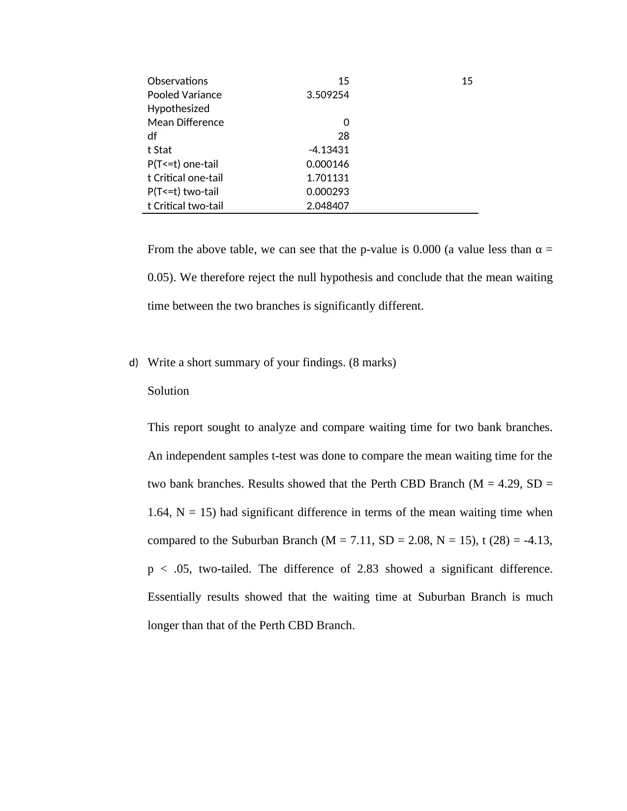
t-Test: Two-Sample Assuming Equal Variances
Perth CBD Branch
(Waiting Time-in
minutes)
Suburban Branch
(Waiting Time-in
minutes)
Mean 4.286667 7.114667
Variance 2.682995 4.335512

Observations 15 15
Pooled Variance 3.509254
Hypothesized
Mean Difference 0
df 28
t Stat -4.13431
P(T<=t) one-tail 0.000146
t Critical one-tail 1.701131
P(T<=t) two-tail 0.000293
t Critical two-tail 2.048407
From the above table, we can see that the p-value is 0.000 (a value less than α =
0.05). We therefore reject the null hypothesis and conclude that the mean waiting
time between the two branches is significantly different.
d) Write a short summary of your findings. (8 marks)
Solution
This report sought to analyze and compare waiting time for two bank branches.
An independent samples t-test was done to compare the mean waiting time for the
two bank branches. Results showed that the Perth CBD Branch (M = 4.29, SD =
1.64, N = 15) had significant difference in terms of the mean waiting time when
compared to the Suburban Branch (M = 7.11, SD = 2.08, N = 15), t (28) = -4.13,
p < .05, two-tailed. The difference of 2.83 showed a significant difference.
Essentially results showed that the waiting time at Suburban Branch is much
longer than that of the Perth CBD Branch.