Quantitative Techniques for MBA Assignment

MBA-QUANTITATIVE
TECHNIQUES

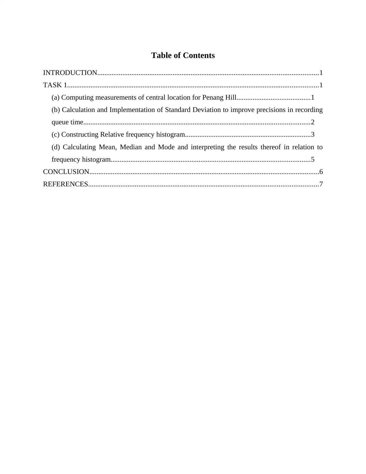
Table of Contents
INTRODUCTION...........................................................................................................................1
TASK 1............................................................................................................................................1
(a) Computing measurements of central location for Penang Hill.........................................1
(b) Calculation and Implementation of Standard Deviation to improve precisions in recording
queue time..............................................................................................................................2
(c) Constructing Relative frequency histogram......................................................................3
(d) Calculating Mean, Median and Mode and interpreting the results thereof in relation to
frequency histogram...............................................................................................................5
CONCLUSION................................................................................................................................6
REFERENCES................................................................................................................................7

INTRODUCTION
Quantitative techniques include statistical or numerical methods to determine whether the
collected data is meaningful for the purpose of deriving conclusions or not. The given report
focuses on the measures of central tendency, dispersion, construction of histogram based on
relative frequencies to interpret results for Penang Hill.
TASK 1
(a) Computing measurements of central location for Penang Hill
A measurement of central location refers to a unit value representative of an entire data
set through identification of a key position within the given set of data. It usually includes Mean,
Median and Mode as three valid measures of central tendency (Asmus and Radocy, 2017).
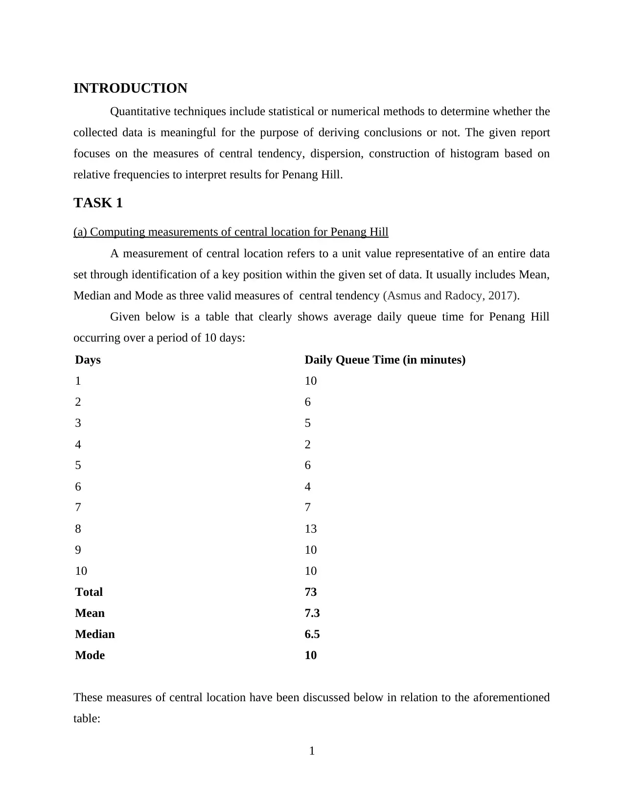
Given below is a table that clearly shows average daily queue time for Penang Hill
occurring over a period of 10 days:
Days Daily Queue Time (in minutes)
1 10
2 6
3 5
4 2
5 6
6 4
7 7
8 13
9 10
10 10
Total 73
Mean 7.3
Median 6.5
Mode 10
These measures of central location have been discussed below in relation to the aforementioned
table:
1

 Mean:
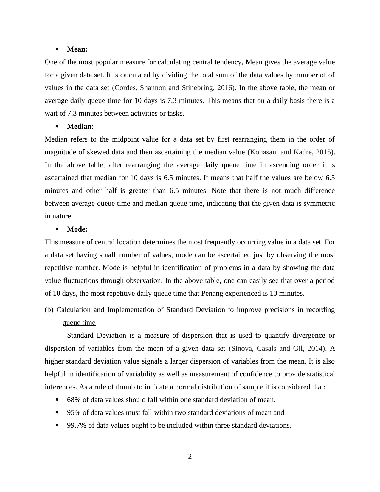
One of the most popular measure for calculating central tendency, Mean gives the average value
for a given data set. It is calculated by dividing the total sum of the data values by number of of
values in the data set (Cordes, Shannon and Stinebring, 2016). In the above table, the mean or
average daily queue time for 10 days is 7.3 minutes. This means that on a daily basis there is a
wait of 7.3 minutes between activities or tasks.
 Median:
Median refers to the midpoint value for a data set by first rearranging them in the order of
magnitude of skewed data and then ascertaining the median value (Konasani and Kadre, 2015).
In the above table, after rearranging the average daily queue time in ascending order it is
ascertained that median for 10 days is 6.5 minutes. It means that half the values are below 6.5
minutes and other half is greater than 6.5 minutes. Note that there is not much difference
between average queue time and median queue time, indicating that the given data is symmetric
in nature.
 Mode:
This measure of central location determines the most frequently occurring value in a data set. For
a data set having small number of values, mode can be ascertained just by observing the most
repetitive number. Mode is helpful in identification of problems in a data by showing the data
value fluctuations through observation. In the above table, one can easily see that over a period
of 10 days, the most repetitive daily queue time that Penang experienced is 10 minutes.
(b) Calculation and Implementation of Standard Deviation to improve precisions in recording
queue time
Standard Deviation is a measure of dispersion that is used to quantify divergence or
dispersion of variables from the mean of a given data set (Sinova, Casals and Gil, 2014). A
higher standard deviation value signals a larger dispersion of variables from the mean. It is also
helpful in identification of variability as well as measurement of confidence to provide statistical
inferences. As a rule of thumb to indicate a normal distribution of sample it is considered that:
 68% of data values should fall within one standard deviation of mean.
 95% of data values must fall within two standard deviations of mean and
 99.7% of data values ought to be included within three standard deviations.
2

Standard Deviation is computed by taking the square root of variance occurring in a set of data
where variance is sum of squared differences of data point from mean divided by number of
variables.
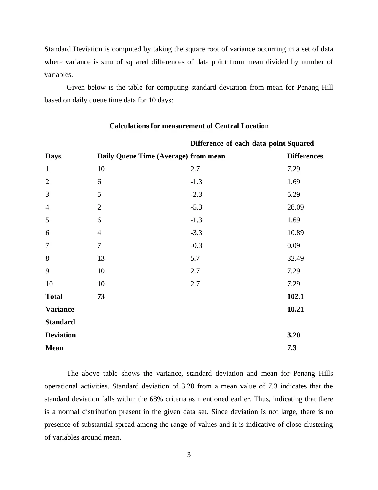
Given below is the table for computing standard deviation from mean for Penang Hill
based on daily queue time data for 10 days:
Calculations for measurement of Central Location
Days Daily Queue Time (Average)
Difference of each data point
from mean
Squared
Differences
1 10 2.7 7.29
2 6 -1.3 1.69
3 5 -2.3 5.29
4 2 -5.3 28.09
5 6 -1.3 1.69
6 4 -3.3 10.89
7 7 -0.3 0.09
8 13 5.7 32.49
9 10 2.7 7.29
10 10 2.7 7.29
Total 73 102.1
Variance 10.21
Standard
Deviation 3.20
Mean 7.3
The above table shows the variance, standard deviation and mean for Penang Hills
operational activities. Standard deviation of 3.20 from a mean value of 7.3 indicates that the
standard deviation falls within the 68% criteria as mentioned earlier. Thus, indicating that there
is a normal distribution present in the given data set. Since deviation is not large, there is no
presence of substantial spread among the range of values and it is indicative of close clustering
of variables around mean.
3

Implementation of this measure is helpful in understanding how significant the
fluctuations are in the data set thus providing the user with information through which it can be
ascertained why these dispersions, large or small, tend to occur and how they can be controlled.
(c) Constructing Relative frequency histogram
In statistics, data may be grouped or disseminated. For grouped data, class width is
clearly defined within which a range of values known as frequency fall. On the other hand,
disseminated data does not include any class width usually containing single random variables as
sample in a given data set.
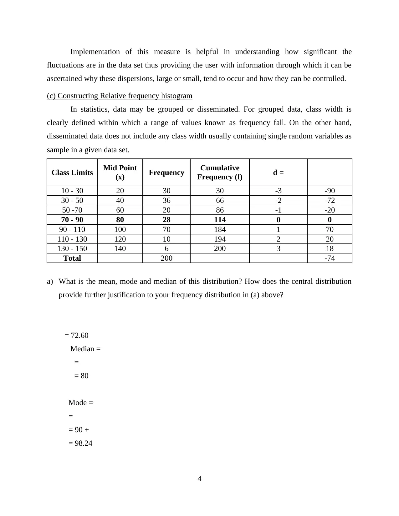
Class Limits Mid Point
(x) Frequency Cumulative
Frequency (f) d =
10 - 30 20 30 30 -3 -90
30 - 50 40 36 66 -2 -72
50 -70 60 20 86 -1 -20
70 - 90 80 28 114 0 0
90 - 110 100 70 184 1 70
110 - 130 120 10 194 2 20
130 - 150 140 6 200 3 18
Total 200 -74
a) What is the mean, mode and median of this distribution? How does the central distribution
provide further justification to your frequency distribution in (a) above?
= 72.60
Median =
=
= 80
Mode =
=
= 90 +
= 98.24
4

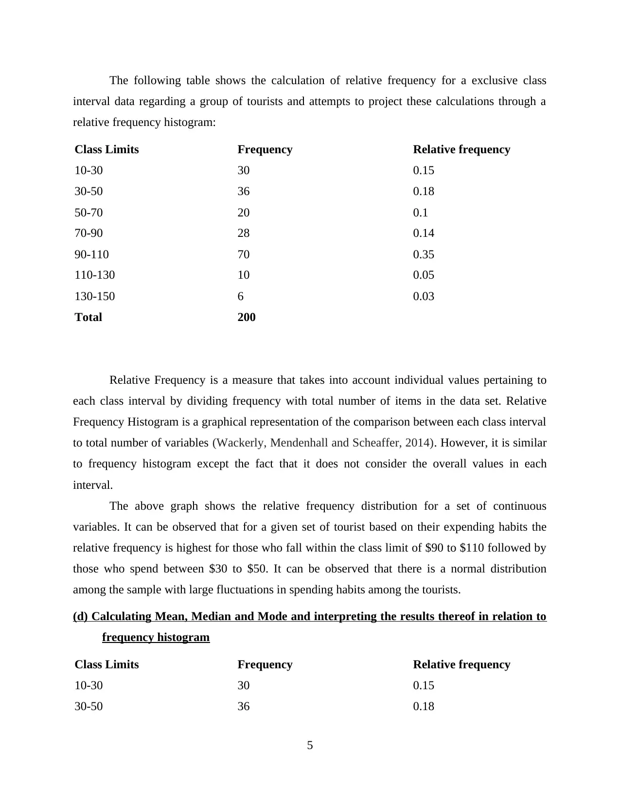
The following table shows the calculation of relative frequency for a exclusive class
interval data regarding a group of tourists and attempts to project these calculations through a
relative frequency histogram:
Class Limits Frequency Relative frequency
10-30 30 0.15
30-50 36 0.18
50-70 20 0.1
70-90 28 0.14
90-110 70 0.35
110-130 10 0.05
130-150 6 0.03
Total 200
Relative Frequency is a measure that takes into account individual values pertaining to
each class interval by dividing frequency with total number of items in the data set. Relative
Frequency Histogram is a graphical representation of the comparison between each class interval
to total number of variables (Wackerly, Mendenhall and Scheaffer, 2014). However, it is similar
to frequency histogram except the fact that it does not consider the overall values in each
interval.
The above graph shows the relative frequency distribution for a set of continuous
variables. It can be observed that for a given set of tourist based on their expending habits the
relative frequency is highest for those who fall within the class limit of $90 to $110 followed by
those who spend between $30 to $50. It can be observed that there is a normal distribution
among the sample with large fluctuations in spending habits among the tourists.
(d) Calculating Mean, Median and Mode and interpreting the results thereof in relation to
frequency histogram
Class Limits Frequency Relative frequency
10-30 30 0.15
30-50 36 0.18
5

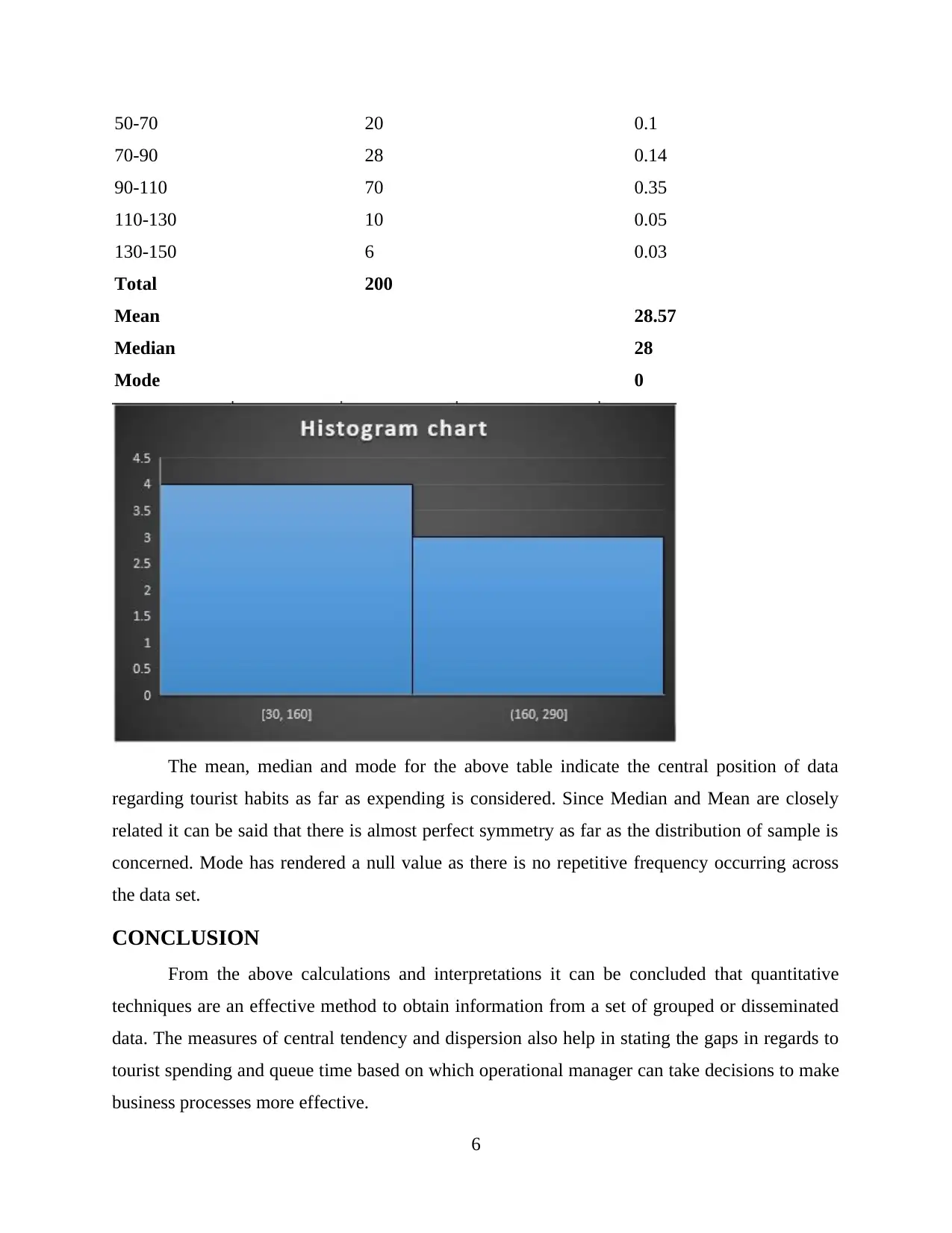
50-70 20 0.1
70-90 28 0.14
90-110 70 0.35
110-130 10 0.05
130-150 6 0.03
Total 200
Mean 28.57
Median 28
Mode 0
The mean, median and mode for the above table indicate the central position of data
regarding tourist habits as far as expending is considered. Since Median and Mean are closely
related it can be said that there is almost perfect symmetry as far as the distribution of sample is
concerned. Mode has rendered a null value as there is no repetitive frequency occurring across
the data set.
CONCLUSION
From the above calculations and interpretations it can be concluded that quantitative
techniques are an effective method to obtain information from a set of grouped or disseminated
data. The measures of central tendency and dispersion also help in stating the gaps in regards to
tourist spending and queue time based on which operational manager can take decisions to make
business processes more effective.
6

REFERENCES
Books and Journal
Asmus, E. P. and Radocy, R. E., 2017. Quantitative analysis. In Critical Essays in Music
Education (pp. 129-172). Routledge.
Cordes, J. M., Shannon, R. M. and Stinebring, D. R., 2016. Frequency-dependent dispersion
measures and implications for pulsar timing. The Astrophysical Journal. 817(1). p.16.
Konasani, V. R. and Kadre, S., 2015. Introduction to business analytics and data analysis tools.
In Practical Business Analytics Using SAS (pp. 3-28). Apress, Berkeley, CA.
Sinova, B., Casals, M. R. and Gil, M. Á., 2014. Central tendency for symmetric random fuzzy
numbers. Information Sciences.278. pp.599-613.
Wackerly, D., Mendenhall, W. and Scheaffer, R. L., 2014. Mathematical statistics with
applications. Cengage Learning.
7