Quantitative Methods for Business

This report explores the application of quantitative methods in solving business problems. It covers topics such as descriptive statistics, regression analysis, and probability. The report also discusses sampling methods and constructing cumulative frequency distributions. The content is relevant for students studying quantitative methods in business.

Quantitive methods for
Business
1

Contents
INTRODUCTION...........................................................................................................................1
QUESTION 1..................................................................................................................................1
(a) An analysis of access time.....................................................................................................1
(b) Sampling methods..................................................................................................................3
(c) Constructing a cumulative frequency distribution.................................................................6
QUESTION 2..................................................................................................................................7
(a) Explanation of the meaning of four regression coefficients..................................................7
(b) Choice related to selection of company along with its reason...............................................8
(c) Expected total running cost for five of the cars in the new region.........................................9
QUESTION 3................................................................................................................................10
(a) Calculating the probability for Chris, Albert, and John.......................................................10
(b) Calculating the probability for box A and box B.................................................................11
CONCLUSION..............................................................................................................................12
REFERENCES..............................................................................................................................13
2

INTRODUCTION
Quantitative methods are the techniques which are used by a business organisation to control
and manage their operations. There are various Quantitative methods and some of them are
project management, probability, forecasting, descriptive and data mining (Mital and et.al,
2015). The main aim of this report is to develop an ability to apply these models and techniques
into solving problems and enhancing decision making power. In this report 3 distinct questions
are resolved using Quantitative methods.
In first question, descriptive statistics tools such as mean and standard deviation are used
along with sampling methods so that data can be effectively analysed and interpreted. In second
question, the Quantitative methods of regression are used. And lastly, in third question the model
of probability is used.
QUESTION 1
(a) An analysis of access time
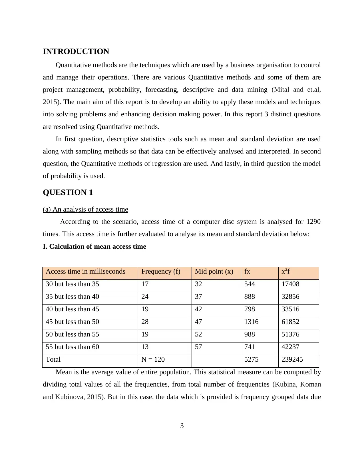
According to the scenario, access time of a computer disc system is analysed for 1290
times. This access time is further evaluated to analyse its mean and standard deviation below:
I. Calculation of mean access time
Access time in milliseconds Frequency (f) Mid point (x) fx x2f
30 but less than 35 17 32 544 17408
35 but less than 40 24 37 888 32856
40 but less than 45 19 42 798 33516
45 but less than 50 28 47 1316 61852
50 but less than 55 19 52 988 51376
55 but less than 60 13 57 741 42237
Total N = 120 5275 239245
Mean is the average value of entire population. This statistical measure can be computed by
dividing total values of all the frequencies, from total number of frequencies (Kubina, Koman
and Kubinova, 2015). But in this case, the data which is provided is frequency grouped data due
3

to which mid points for each group is calculated and then the sum of midpoint and frequency is
divided by the sum of all frequencies. Average access time is calculated as follows.
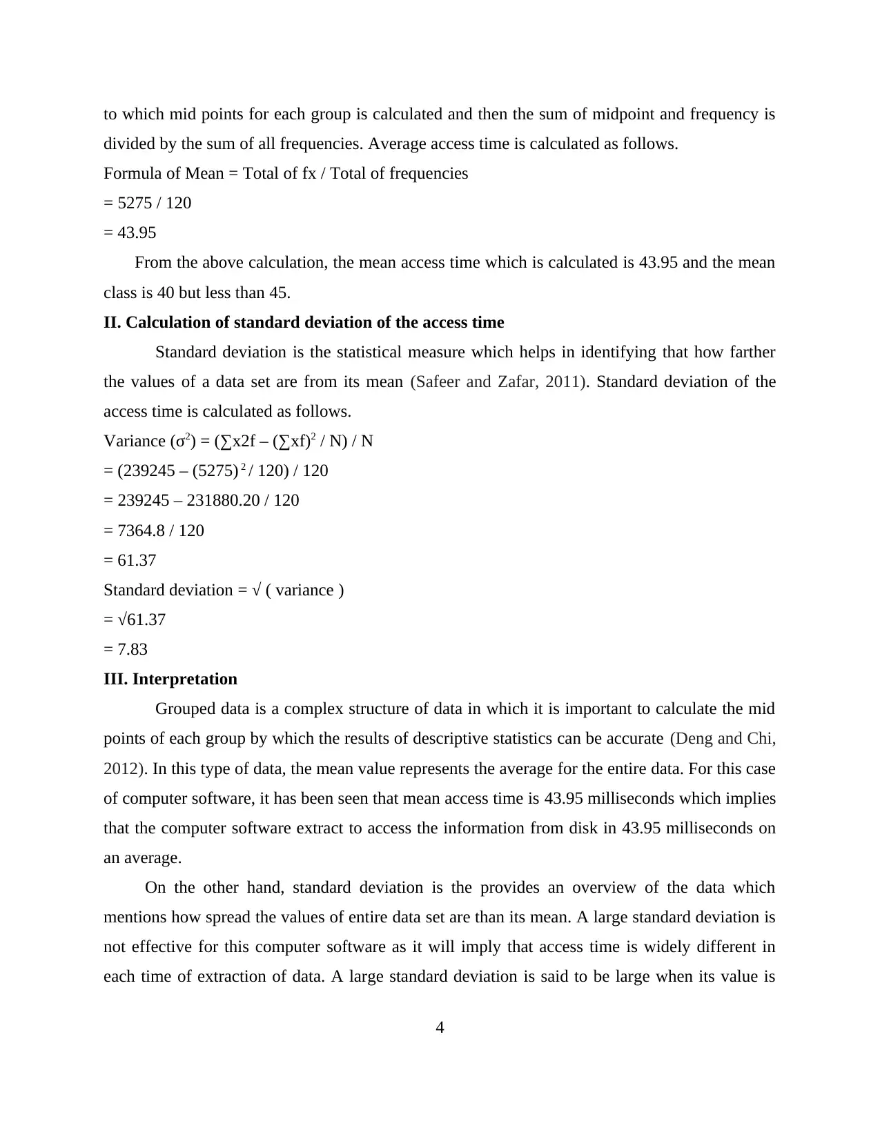
Formula of Mean = Total of fx / Total of frequencies
= 5275 / 120
= 43.95
From the above calculation, the mean access time which is calculated is 43.95 and the mean
class is 40 but less than 45.
II. Calculation of standard deviation of the access time
Standard deviation is the statistical measure which helps in identifying that how farther
the values of a data set are from its mean (Safeer and Zafar, 2011). Standard deviation of the
access time is calculated as follows.
Variance (σ2) = (∑x2f – (∑xf)2 / N) / N
= (239245 – (5275) 2 / 120) / 120
= 239245 – 231880.20 / 120
= 7364.8 / 120
= 61.37
Standard deviation = √ ( variance )
= √61.37
= 7.83
III. Interpretation
Grouped data is a complex structure of data in which it is important to calculate the mid
points of each group by which the results of descriptive statistics can be accurate (Deng and Chi,
2012). In this type of data, the mean value represents the average for the entire data. For this case
of computer software, it has been seen that mean access time is 43.95 milliseconds which implies
that the computer software extract to access the information from disk in 43.95 milliseconds on
an average.
On the other hand, standard deviation is the provides an overview of the data which
mentions how spread the values of entire data set are than its mean. A large standard deviation is
not effective for this computer software as it will imply that access time is widely different in
each time of extraction of data. A large standard deviation is said to be large when its value is
4

more than its mean. In this case, the standard deviation is 7.83 milliseconds which is lower than
the mean that implies, in this case all the access times are clustered to its mean.
To sum it up, it can be said that average access time taken by the computer disc system is
43.95 milliseconds with plus minus of 7.83 milliseconds.
(b) Sampling methods
The concept of sampling is the procedure of selecting a subset of data from the entire
population of data. There are various ways by which sampling can be done and which are known
as sampling methods. Each sampling method is appropriate according to the desired outcomes.
Four of these methods are analysed below along with a practical example for each.
i. Simple random sampling
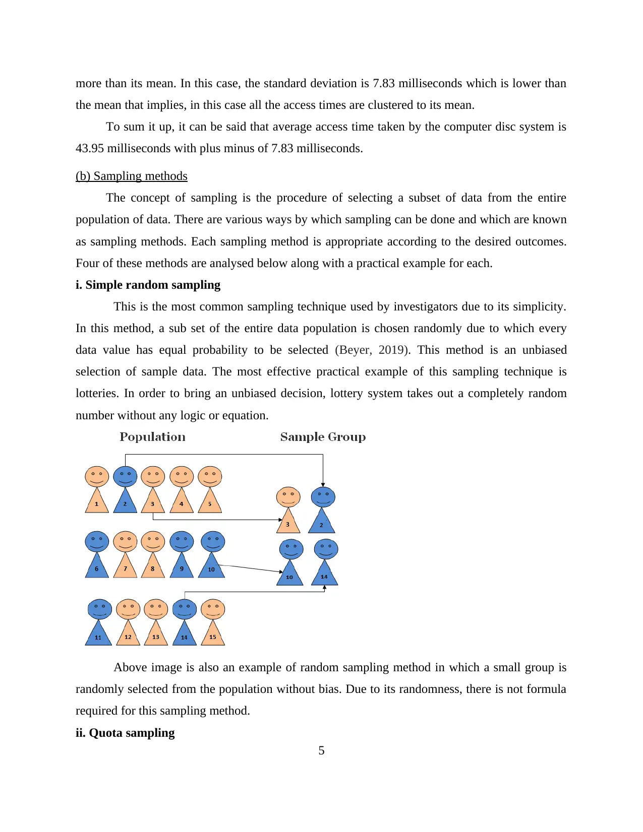
This is the most common sampling technique used by investigators due to its simplicity.
In this method, a sub set of the entire data population is chosen randomly due to which every
data value has equal probability to be selected (Beyer, 2019). This method is an unbiased
selection of sample data. The most effective practical example of this sampling technique is
lotteries. In order to bring an unbiased decision, lottery system takes out a completely random
number without any logic or equation.
Above image is also an example of random sampling method in which a small group is
randomly selected from the population without bias. Due to its randomness, there is not formula
required for this sampling method.
ii. Quota sampling
5

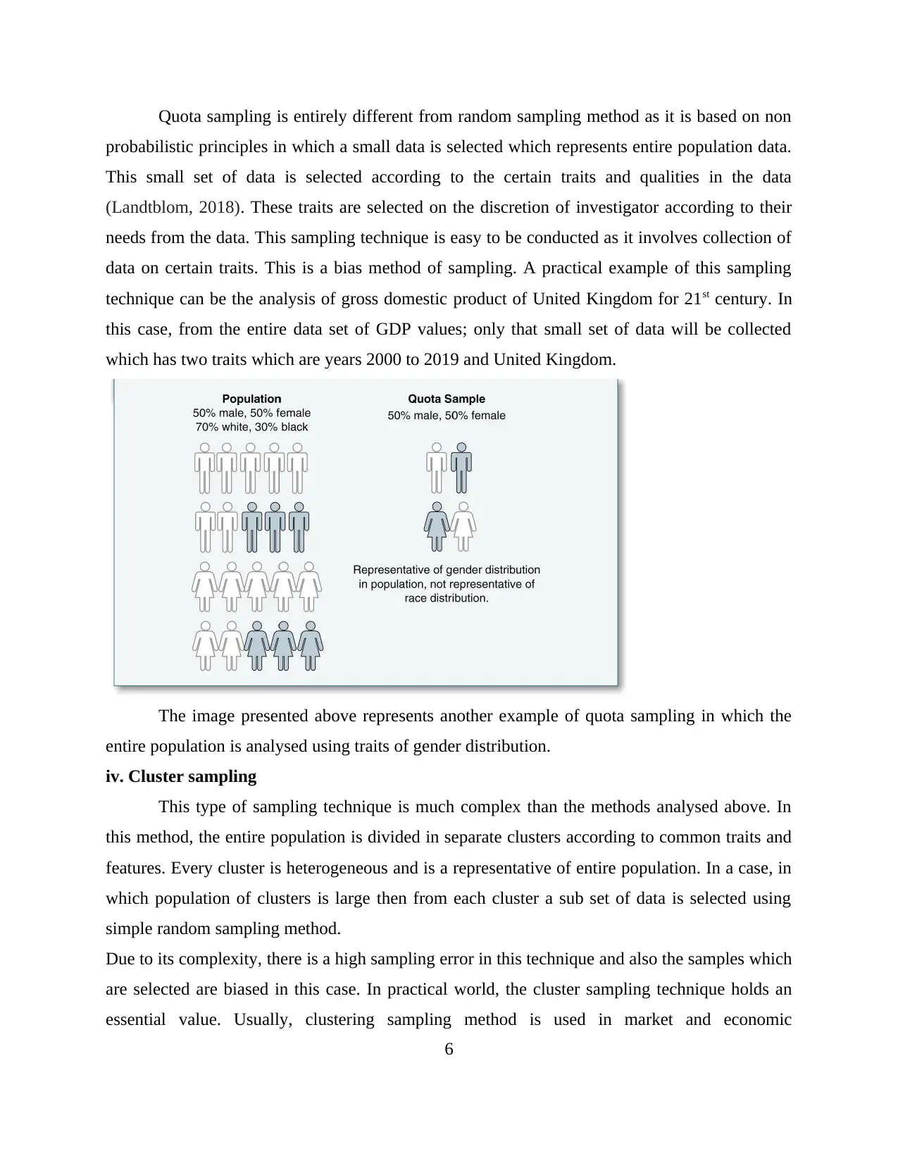
Quota sampling is entirely different from random sampling method as it is based on non
probabilistic principles in which a small data is selected which represents entire population data.
This small set of data is selected according to the certain traits and qualities in the data
(Landtblom, 2018). These traits are selected on the discretion of investigator according to their
needs from the data. This sampling technique is easy to be conducted as it involves collection of
data on certain traits. This is a bias method of sampling. A practical example of this sampling
technique can be the analysis of gross domestic product of United Kingdom for 21st century. In
this case, from the entire data set of GDP values; only that small set of data will be collected
which has two traits which are years 2000 to 2019 and United Kingdom.
The image presented above represents another example of quota sampling in which the
entire population is analysed using traits of gender distribution.
iv. Cluster sampling
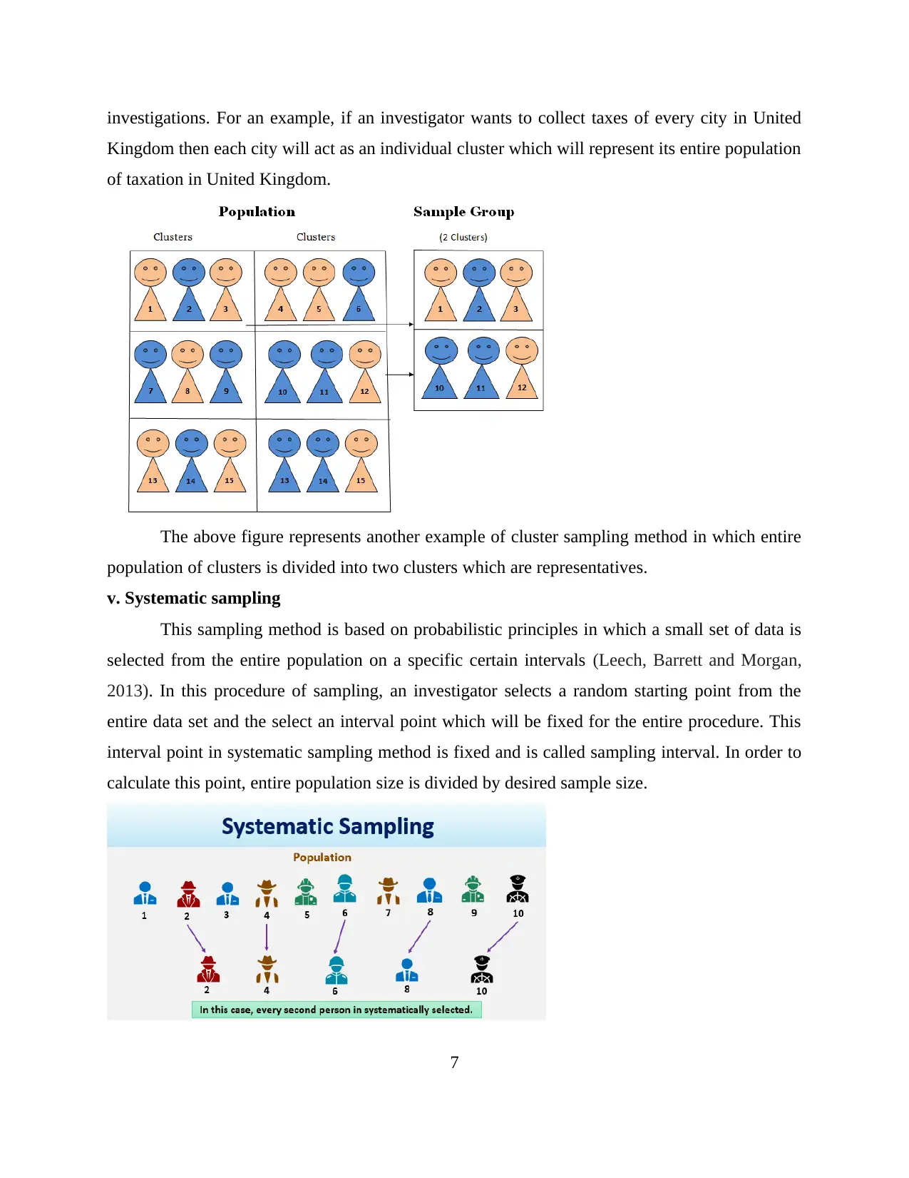
This type of sampling technique is much complex than the methods analysed above. In
this method, the entire population is divided in separate clusters according to common traits and
features. Every cluster is heterogeneous and is a representative of entire population. In a case, in
which population of clusters is large then from each cluster a sub set of data is selected using
simple random sampling method.
Due to its complexity, there is a high sampling error in this technique and also the samples which
are selected are biased in this case. In practical world, the cluster sampling technique holds an
essential value. Usually, clustering sampling method is used in market and economic
6

investigations. For an example, if an investigator wants to collect taxes of every city in United
Kingdom then each city will act as an individual cluster which will represent its entire population
of taxation in United Kingdom.
The above figure represents another example of cluster sampling method in which entire
population of clusters is divided into two clusters which are representatives.
v. Systematic sampling
This sampling method is based on probabilistic principles in which a small set of data is
selected from the entire population on a specific certain intervals (Leech, Barrett and Morgan,
2013). In this procedure of sampling, an investigator selects a random starting point from the
entire data set and the select an interval point which will be fixed for the entire procedure. This
interval point in systematic sampling method is fixed and is called sampling interval. In order to
calculate this point, entire population size is divided by desired sample size.
7

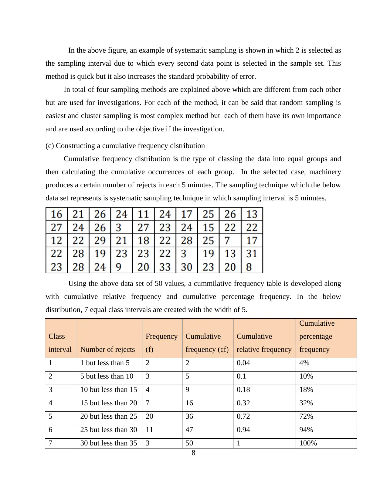
In the above figure, an example of systematic sampling is shown in which 2 is selected as
the sampling interval due to which every second data point is selected in the sample set. This
method is quick but it also increases the standard probability of error.
In total of four sampling methods are explained above which are different from each other
but are used for investigations. For each of the method, it can be said that random sampling is
easiest and cluster sampling is most complex method but each of them have its own importance
and are used according to the objective if the investigation.
(c) Constructing a cumulative frequency distribution
Cumulative frequency distribution is the type of classing the data into equal groups and
then calculating the cumulative occurrences of each group. In the selected case, machinery
produces a certain number of rejects in each 5 minutes. The sampling technique which the below
data set represents is systematic sampling technique in which sampling interval is 5 minutes.
Using the above data set of 50 values, a cummilative frequency table is developed along
with cumulative relative frequency and cumulative percentage frequency. In the below
distribution, 7 equal class intervals are created with the width of 5.
Class
interval Number of rejects
Frequency
(f)
Cumulative
frequency (cf)
Cumulative
relative frequency
Cumulative
percentage
frequency
1 1 but less than 5 2 2 0.04 4%
2 5 but less than 10 3 5 0.1 10%
3 10 but less than 15 4 9 0.18 18%
4 15 but less than 20 7 16 0.32 32%
5 20 but less than 25 20 36 0.72 72%
6 25 but less than 30 11 47 0.94 94%
7 30 but less than 35 3 50 1 100%
8

QUESTION 2
(a) Explanation of the meaning of four regression coefficients
Car F: y = 2.650 + 0.794 x
Car L: y = 5.585 + 0.427 x
In the above data four different types of regression coefficients are applied which are as
follows:
Coefficient of variation: It is used in the data to analyse the way in which data points are
dispersed around the mean. It is applied in the above data as it is demonstrating the variation
between the values of x and y of Car F and Car L. With the help of it, the researchers can get
accurate results for the hypothesis which is formulated by them to resolve their queries. Main use
of it is to demonstrate the extent of variability of data in the sample.
Coefficient of determination: In the above data this coefficient is also applied as it helps
to assess the way in which variation in one variable could be explained from the difference in
another variable. In order to find the causes of variability in the value of X and Y of Car F and
Car L this coefficient is applied to the data. In regression it is used to analyse the goodness of fit
and represented as value between 0 to 1 (Cleophas and Zwinderman, 2016).
Coefficient of dispersion: This coefficient is mainly used for the purpose of analysing
and measuring dispersions in the statistics. In the above data it is used to determine the
dispersion in the regression so that accurate results could be developed. Main use of it is to
appraise uniformity and express the percentage of the deviation of the data series. While dealing
with densities this coefficient is figured out.
Multinomial coefficient: In case of duplicate or repeating values this coefficient is used
to figure out permutations. In the above data it is applied because in the data series which is
provided in the example having various values which are repeating. To ignore the complexities
in the calculations it is applied in the data set and then results are generated (Kaengthong and
Domthong, 2017).
9

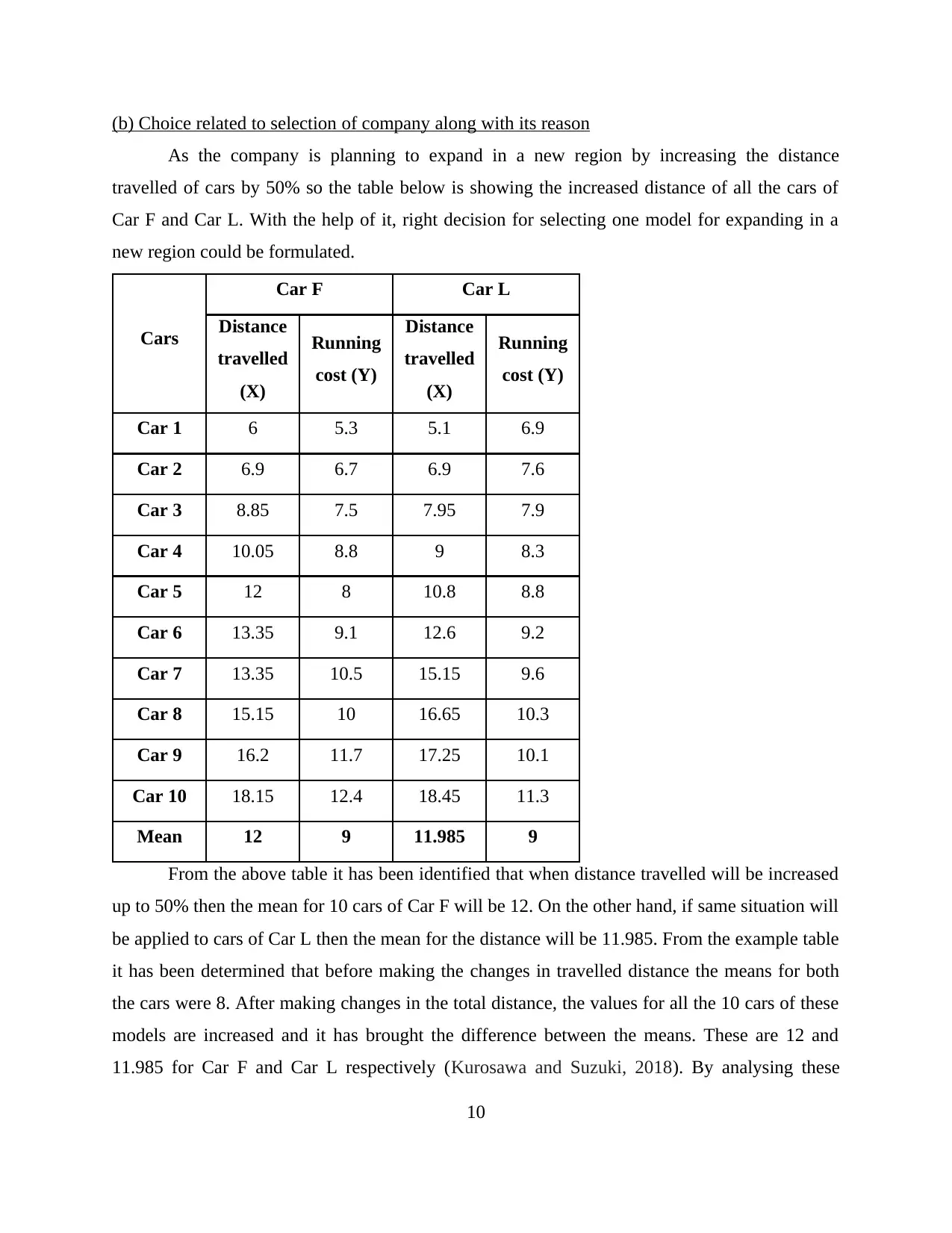
(b) Choice related to selection of company along with its reason
As the company is planning to expand in a new region by increasing the distance
travelled of cars by 50% so the table below is showing the increased distance of all the cars of
Car F and Car L. With the help of it, right decision for selecting one model for expanding in a
new region could be formulated.
Cars
Car F Car L
Distance
travelled
(X)
Running
cost (Y)
Distance
travelled
(X)
Running
cost (Y)
Car 1 6 5.3 5.1 6.9
Car 2 6.9 6.7 6.9 7.6
Car 3 8.85 7.5 7.95 7.9
Car 4 10.05 8.8 9 8.3
Car 5 12 8 10.8 8.8
Car 6 13.35 9.1 12.6 9.2
Car 7 13.35 10.5 15.15 9.6
Car 8 15.15 10 16.65 10.3
Car 9 16.2 11.7 17.25 10.1
Car 10 18.15 12.4 18.45 11.3
Mean 12 9 11.985 9
From the above table it has been identified that when distance travelled will be increased
up to 50% then the mean for 10 cars of Car F will be 12. On the other hand, if same situation will
be applied to cars of Car L then the mean for the distance will be 11.985. From the example table
it has been determined that before making the changes in travelled distance the means for both
the cars were 8. After making changes in the total distance, the values for all the 10 cars of these
models are increased and it has brought the difference between the means. These are 12 and
11.985 for Car F and Car L respectively (Kurosawa and Suzuki, 2018). By analysing these
10

changes, it has been recommended to the organisation that it should choose the first car for the
new region in which it is planning for expansion. The main reason for the same is higher mean of
the first car. There is a slight difference in the mean but if the company is willing to choose only
one car then it should be Car F. If the company will select Car L then it will not make higher
difference but if first option will be selected then there is a possibility of generating higher
revenues in the new region.
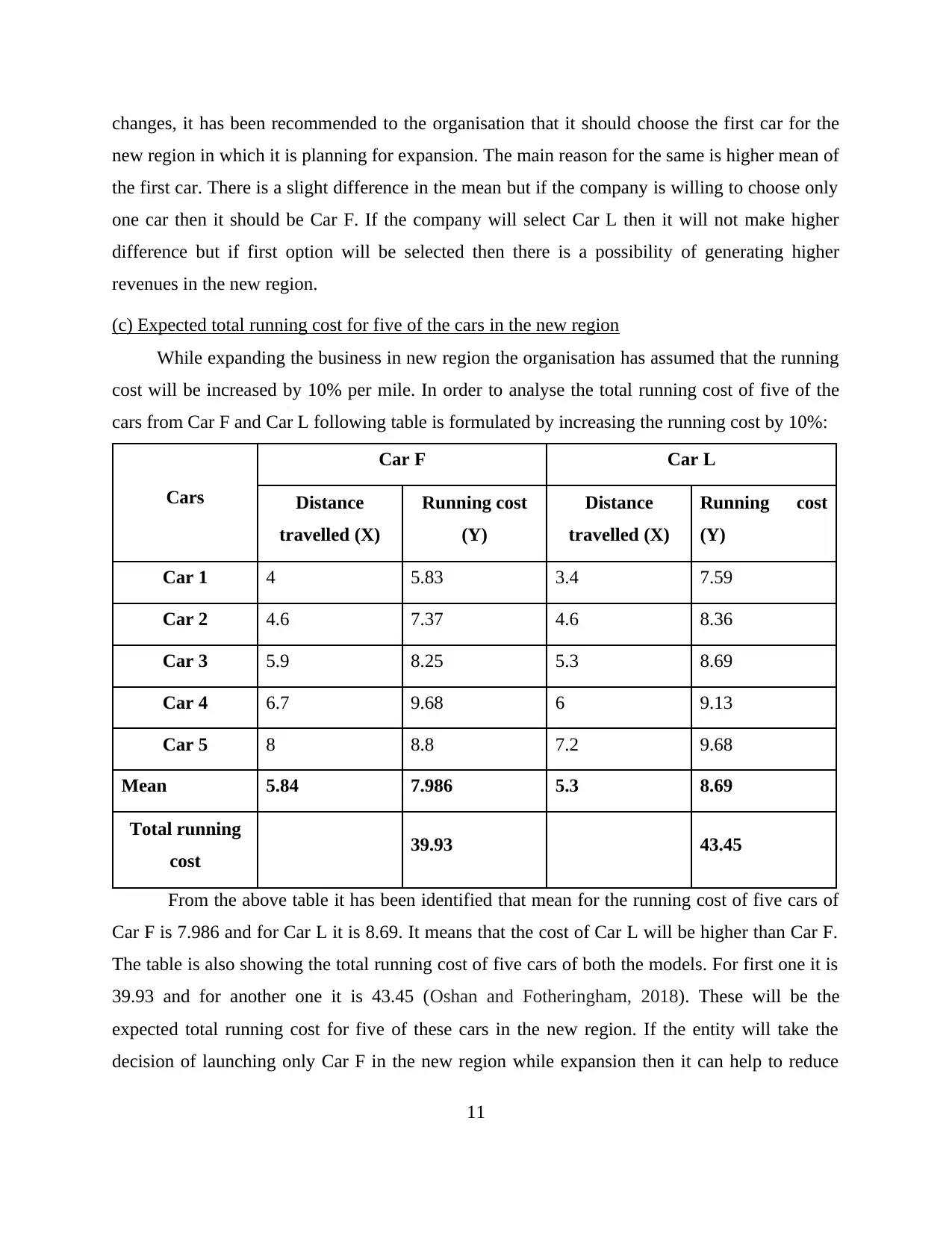
(c) Expected total running cost for five of the cars in the new region
While expanding the business in new region the organisation has assumed that the running
cost will be increased by 10% per mile. In order to analyse the total running cost of five of the
cars from Car F and Car L following table is formulated by increasing the running cost by 10%:
Cars
Car F Car L
Distance
travelled (X)
Running cost
(Y)
Distance
travelled (X)
Running cost
(Y)
Car 1 4 5.83 3.4 7.59
Car 2 4.6 7.37 4.6 8.36
Car 3 5.9 8.25 5.3 8.69
Car 4 6.7 9.68 6 9.13
Car 5 8 8.8 7.2 9.68
Mean 5.84 7.986 5.3 8.69
Total running
cost 39.93 43.45
From the above table it has been identified that mean for the running cost of five cars of
Car F is 7.986 and for Car L it is 8.69. It means that the cost of Car L will be higher than Car F.
The table is also showing the total running cost of five cars of both the models. For first one it is
39.93 and for another one it is 43.45 (Oshan and Fotheringham, 2018). These will be the
expected total running cost for five of these cars in the new region. If the entity will take the
decision of launching only Car F in the new region while expansion then it can help to reduce
11

costs as the cost of Car L is very high. Total cost for F is very low as compared to L therefore if
the entity is planning to introduce only one of them in the new region then it should be Car F.
QUESTION 3
(a) Calculating the probability for Chris, Albert, and John
Probability is the concept of calculating the possibility of occurrences of an event. The value
of probability can be only expressed between 0 to 1 and it helps to predict the exact possibility of
an event to occur (Sarkar and Rashid, 2016). This measure is the likelihood of an event and it can
only be predicted. As it has been known that future is uncertain and probability only helps in
measuring the possibility of occurrences of future events and it does not provide any exact
prediction. The basic formula of calculating probability is to divide number of all favourable
events from number of total events. Besides this, there are various kinds of probability which
helps to analyse single as well as multiple event probability at once. These types of probability
are theoretical, experimental and axiomatic probability. In this case only theoretical and
experimental are used.
According to the given scenario, there are three players in a contest who are Chris, Albert
and John. All these three players have a certain probability to win the contest which is 0.166,
0.125 and 0.33 respectively. Using these probabilities, further probabilities for three events are
calculated as follows.
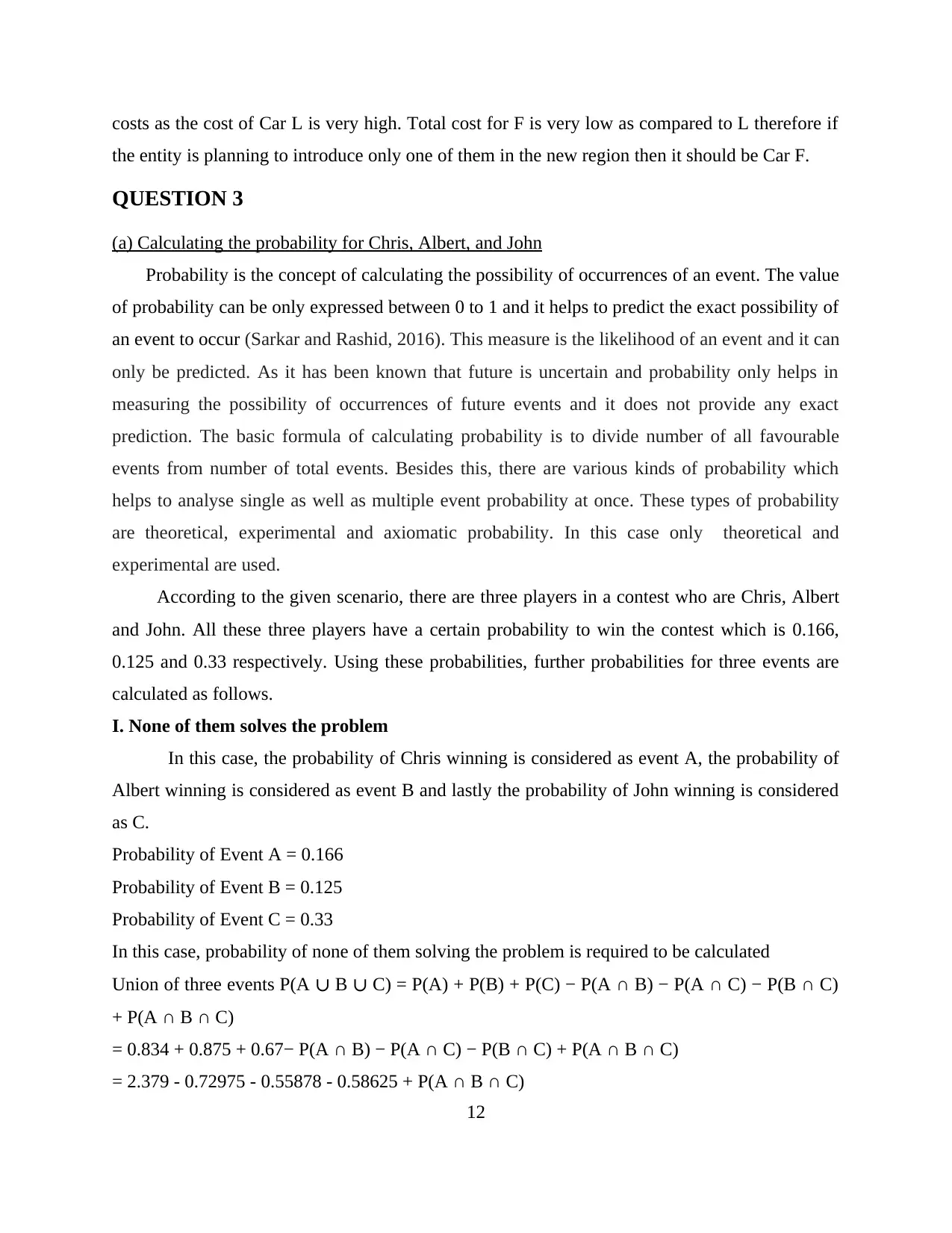
I. None of them solves the problem
In this case, the probability of Chris winning is considered as event A, the probability of
Albert winning is considered as event B and lastly the probability of John winning is considered
as C.
Probability of Event A = 0.166
Probability of Event B = 0.125
Probability of Event C = 0.33
In this case, probability of none of them solving the problem is required to be calculated
Union of three events P(A ∪ B ∪ C) = P(A) + P(B) + P(C) − P(A ∩ B) − P(A ∩ C) − P(B ∩ C)
+ P(A ∩ B ∩ C)
= 0.834 + 0.875 + 0.67− P(A ∩ B) − P(A ∩ C) − P(B ∩ C) + P(A ∩ B ∩ C)
= 2.379 - 0.72975 - 0.55878 - 0.58625 + P(A ∩ B ∩ C)
12

= 0.50422 + (-0.015288)
= 0.488932
II. At least one of them solves the problem
P(AΔB) = P(A) + P(B) + P(C) − P(A ∩ B) − P(A ∩ C) − P(B ∩ C) + Chance of all happening
= 0.488932 + 0.00684750
= 0.511068
III. Only one of them solves the problem
P(AΔB) = P(A) + P(B) + P(C) − P(A ∩ B) − P(A ∩ C) − P(B ∩ C) - Chance of all happening
= 0.488932 - 0.00684750
= 0.407983
(b) Calculating the probability for box A and box B
According to the given scenario, there are two boxes which are A and B. the box A has
total of 5 balls out of which 3 are white and 2 are blue. On the other hand, box B has total of 9
balls out of which 4 are green and 5 are blue. Using this situation, probabilities are calculated as
follows.
I. One is green and the other is white
In this case, the event of getting a green ball from box B is assumed as event A and the
event of getting a white ball from box B is considered as event B.
Probability of Event A = number of favourable events / number of total events
= 4 / 9 = 0.44
Probability of non occurrence of event A = 1 - 0.44 = 0.55
Probability of event B = number of favourable events / number of total events
= 2 / 5 = 0.6
Probability of non occurrence of event B = 1 – 0.6 = 0.4
Probability of event A and B occurring P(A∩B) = P(A) × P(B)
= 0.44444 × 0.6
= 0.26
II. They are of the same colour
13

In this case, both the boxes that is A and B has 2 and 5 blue balls. The event of getting a
blue ball from box A is considered as Event A and the event of getting a blue ball from box B is
considered as Event B.
Probability of Event A = number of favourable events / number of total events
= 2 / 5 = 0.4
Probability of Event B = number of favourable events / number of total events
= 5 / 9 = 0.55
Probability of union of event A and B P(A∩B) = P (A) × P (B)
= 0.4 * 0.55
= 0.22
CONCLUSION
From the above report, it has been concluded that Quantitative methods are the techniques
which are used by a business organisation to make effective decision making. The above report
is the summarisation of various sampling techniques out of which random sampling is analysed
to be simplest and cluster sampling is analysed to be most complex sampling technique. In above
report, probability of various events are calculated from which it has been seen that occurrences
of two events is known as probability but occurrences of three or more events is known as
conjunction. In above report, concept of regression is also analysed from which it has been
analysed that regression is a technique of identifying the relationship between two more
variables along with the strength of their relationship.
14

REFERENCES
Books and Journals
Mital, V., and et.al, 2015. Data mining in a business intelligence document. U.S. Patent
9,110,957.
Kubina, M., Koman, G. and Kubinova, I., 2015. Possibility of improving efficiency within
business intelligence systems in companies. Procedia Economics and Finance. 26.
pp.300-305.
Safeer, M. and Zafar, S., 2011, December. Impact of business intelligence competency center in
success/failure of BI applications. In 2011 IEEE 14th International Multitopic
Conference (pp. 267-272). IEEE.
Deng, X. and Chi, L., 2012. Understanding postadoptive behaviors in information systems use:
A longitudinal analysis of system use problems in the business intelligence
context. Journal of Management Information Systems. 29(3). pp.291-326.
Beyer, W. H., 2019. Handbook of tables for probability and statistics. Crc Press.
Landtblom, K. K., 2018. Prospective Teachers’ Conceptions of the Concepts Mean, Median and
Mode. In Students' and Teachers' Values, Attitudes, Feelings and Beliefs in
Mathematics Classrooms (pp. 43-52). Springer, Cham.
Leech, N., Barrett, K. and Morgan, G. A., 2013. SPSS for intermediate statistics: Use and
interpretation. Routledge.
Sarkar, J. and Rashid, M., 2016. Visualizing mean, median, mean deviation, and standard
deviation of a set of numbers. The American Statistician. 70(3). pp.304-312.
Cleophas, T. J. and Zwinderman, A. H., 2016. Linear Regression (Regression Coefficient,
Correlation Coefficient and Their Standard Errors). In Clinical Data Analysis on a
Pocket Calculator (pp. 45-50). Springer, Cham.
Kaengthong, N. and Domthong, U., 2017, September. Modified Regression Correlation
Coefficient for Poisson Regression Model. In Journal of Physics: Conference
Series (Vol. 890, No. 1, p. 012155). IOP Publishing.
Kurosawa, T. and Suzuki, N., 2018. Asymptotic distribution of regression correlation coefficient
for Poisson regression model. Communications in Statistics-Theory and Methods. 47(1).
pp.166-180.
Oshan, T. M. and Fotheringham, A. S., 2018. A comparison of spatially varying regression
coefficient estimates using geographically weighted and spatial‐filter‐based
techniques. Geographical Analysis. 50(1). pp.53-75.
15