Control Systems: Signal Analysis, System Response, and Discrete Time
VerifiedAdded on 2023/04/25
|8
|1305
|66
Homework Assignment
AI Summary
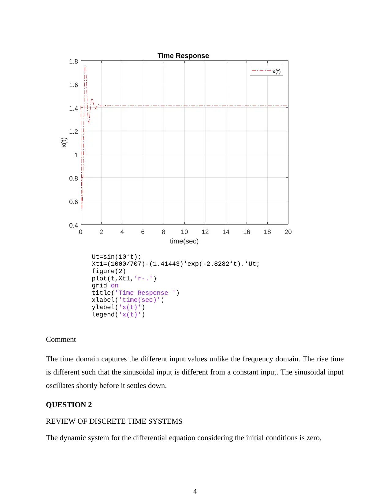
This assignment delves into the analysis of control systems, focusing on signal processing, system responses, and discrete-time systems. It begins with a review of signals and systems, utilizing Laplace transforms to determine time series responses and employing MATLAB for visualization. The impact of varying damping coefficients on system behavior, particularly in the frequency domain, is examined using Bode diagrams and sinusoidal inputs. The assignment then transitions to discrete-time systems, deriving state-space representations and Z-transforms. Finally, it explores least squares solutions for system identification, creating datasets and analyzing parameter estimates. The assignment uses MATLAB extensively to simulate system behavior and validate analytical results. Desklib provides this solved assignment and other resources for students.
1 out of 8
Related Documents


Your All-in-One AI-Powered Toolkit for Academic Success.
+13062052269
info@desklib.com
Available 24*7 on WhatsApp / Email
![[object Object]](/_next/static/media/star-bottom.7253800d.svg)
Copyright © 2020–2026 A2Z Services. All Rights Reserved. Developed and managed by ZUCOL.