Logistic Regression Analysis for Survey Data Variables

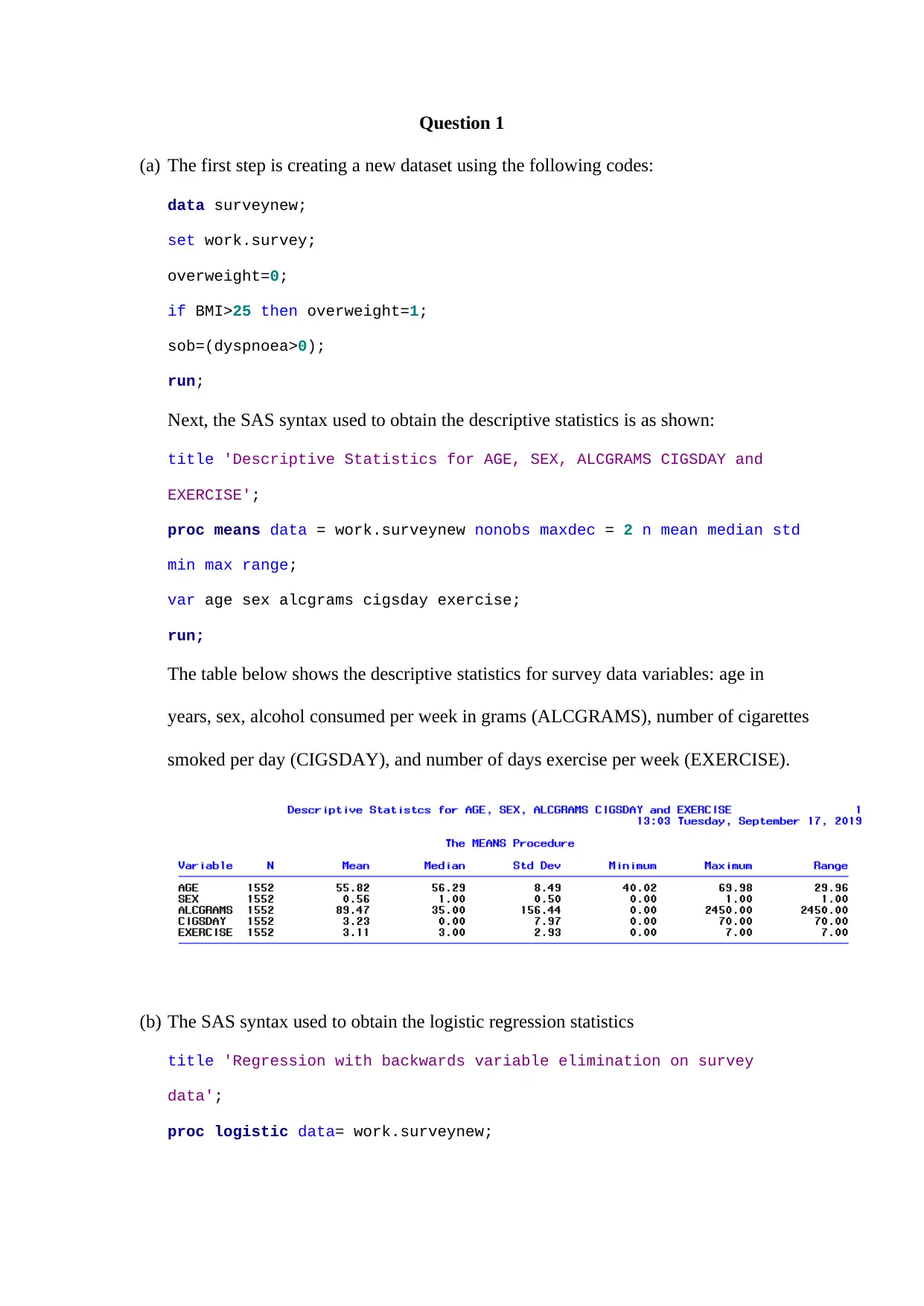
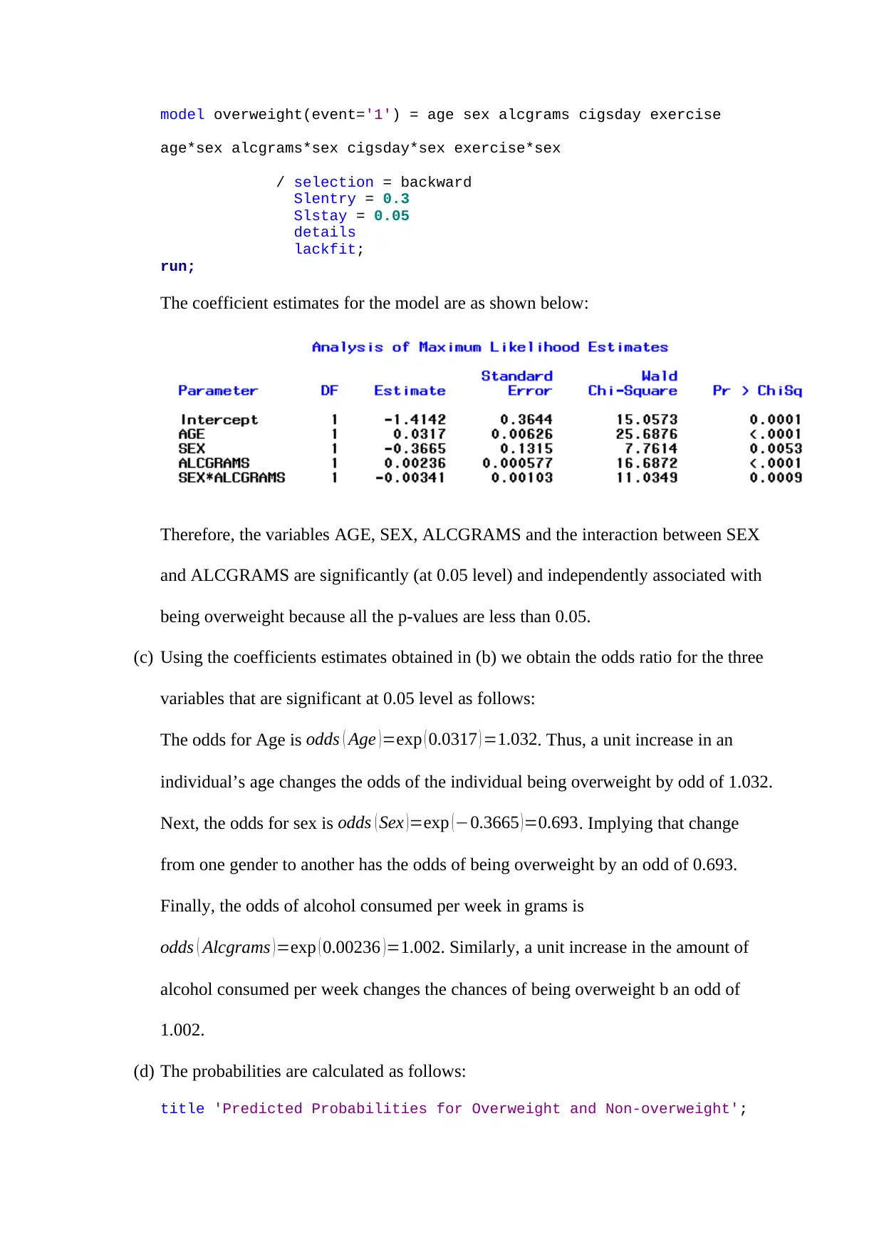
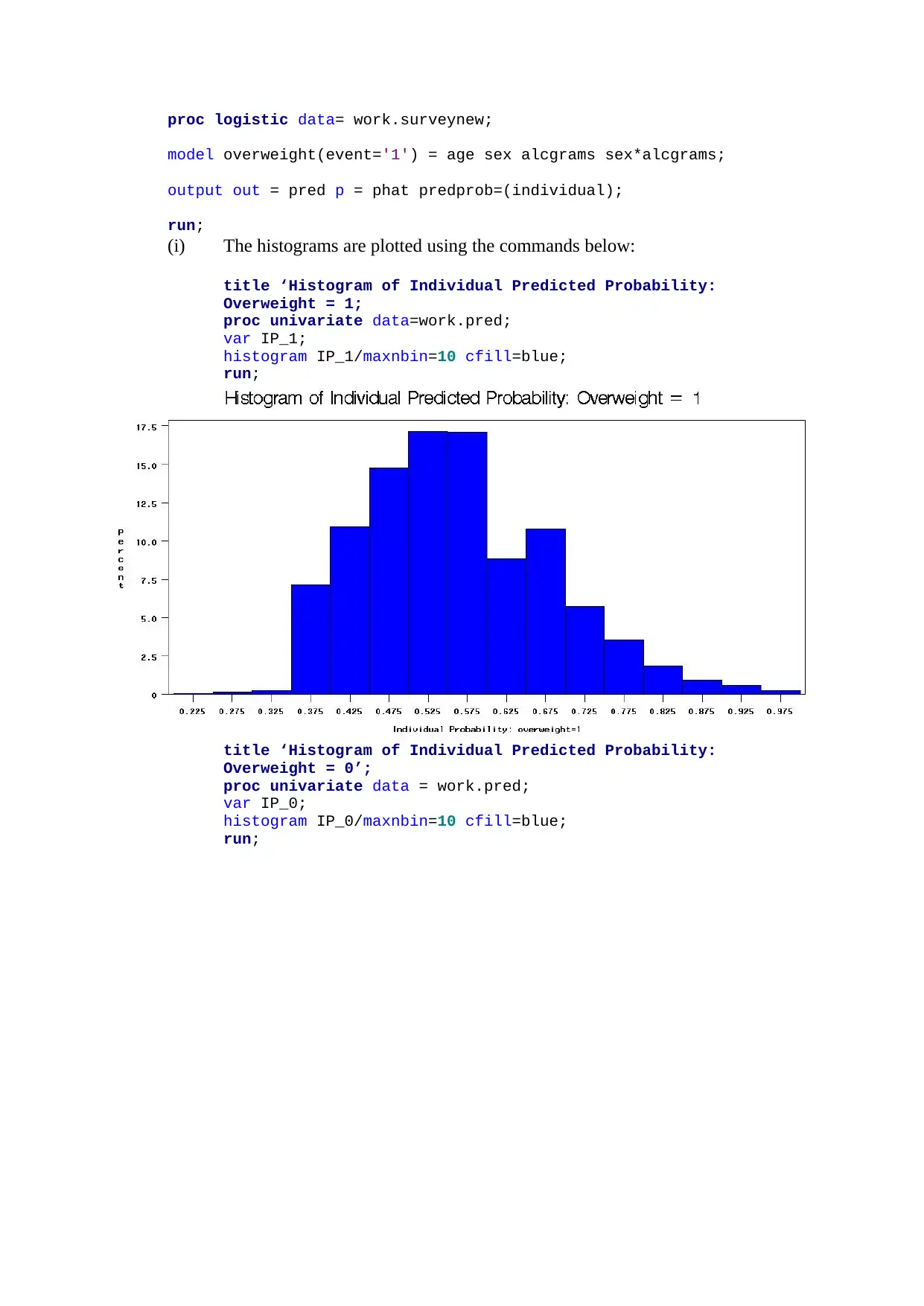
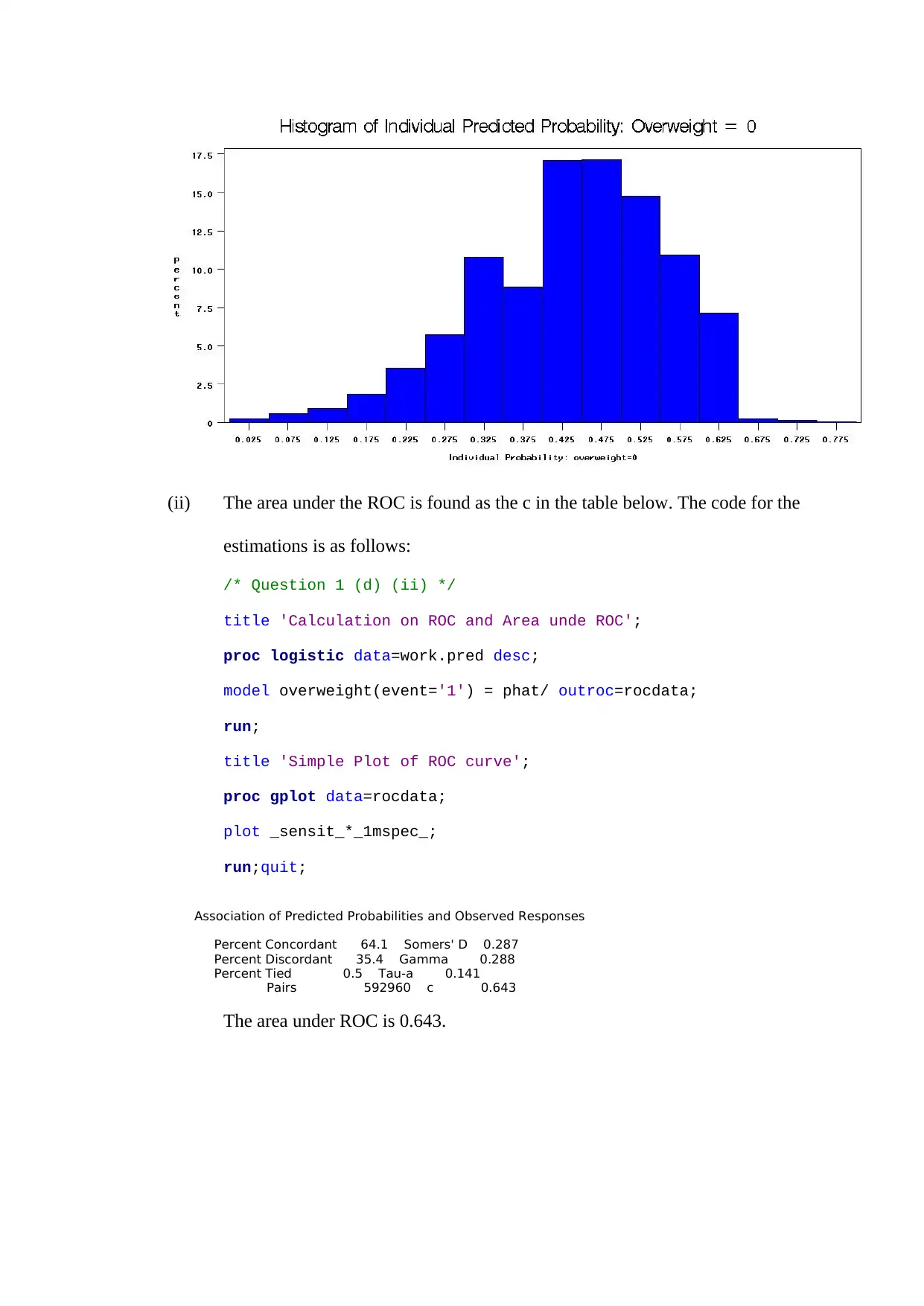
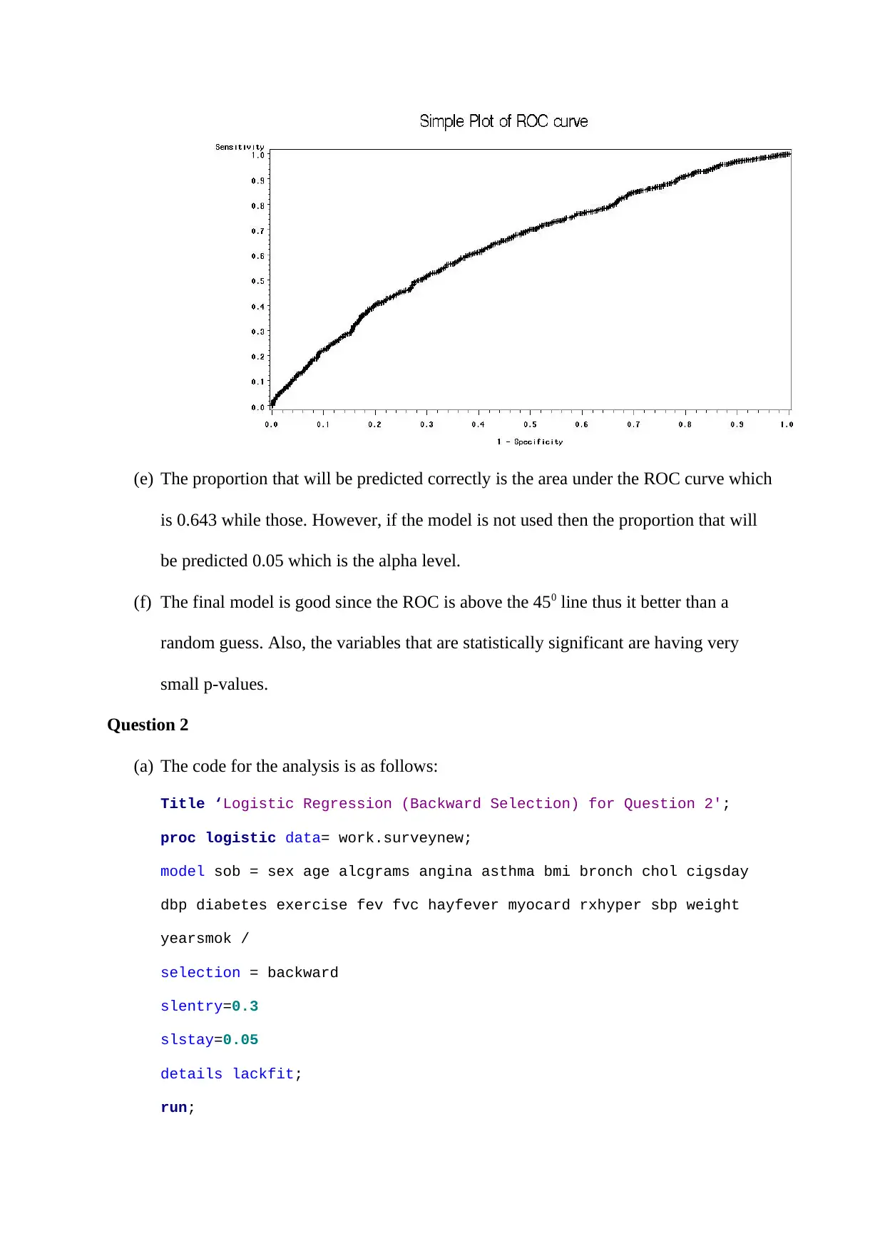
Learn how to perform logistic regression analysis on survey data variables using SAS syntax. Obtain descriptive statistics and coefficient estimates for the model. Find out the odds ratio and predicted probabilities for significant variables. Also, calculate the area under the ROC curve and proportion of correct predictions. Get insights into the analysis of odds for age-stratified case-control study of the association between alcohol consumption and oesophageal cancer in a region of France.

Question 1
(a) The first step is creating a new dataset using the following codes:
data surveynew;
set work.survey;
overweight=0;
if BMI>25 then overweight=1;
sob=(dyspnoea>0);
run;
Next, the SAS syntax used to obtain the descriptive statistics is as shown:
title 'Descriptive Statistics for AGE, SEX, ALCGRAMS CIGSDAY and
EXERCISE';
proc means data = work.surveynew nonobs maxdec = 2 n mean median std
min max range;
var age sex alcgrams cigsday exercise;
run;
The table below shows the descriptive statistics for survey data variables: age in
years, sex, alcohol consumed per week in grams (ALCGRAMS), number of cigarettes
smoked per day (CIGSDAY), and number of days exercise per week (EXERCISE).
(b) The SAS syntax used to obtain the logistic regression statistics
title 'Regression with backwards variable elimination on survey
data';
proc logistic data= work.surveynew;

model overweight(event='1') = age sex alcgrams cigsday exercise
age*sex alcgrams*sex cigsday*sex exercise*sex
/ selection = backward
Slentry = 0.3
Slstay = 0.05
details
lackfit;
run;
The coefficient estimates for the model are as shown below:
Therefore, the variables AGE, SEX, ALCGRAMS and the interaction between SEX
and ALCGRAMS are significantly (at 0.05 level) and independently associated with
being overweight because all the p-values are less than 0.05.
(c) Using the coefficients estimates obtained in (b) we obtain the odds ratio for the three
variables that are significant at 0.05 level as follows:
The odds for Age is odds ( Age )=exp ( 0.0317 ) =1.032. Thus, a unit increase in an
individual’s age changes the odds of the individual being overweight by odd of 1.032.
Next, the odds for sex is odds ( Sex )=exp (−0.3665 )=0.693. Implying that change
from one gender to another has the odds of being overweight by an odd of 0.693.
Finally, the odds of alcohol consumed per week in grams is
odds ( Alcgrams )=exp ( 0.00236 )=1.002. Similarly, a unit increase in the amount of
alcohol consumed per week changes the chances of being overweight b an odd of
1.002.
(d) The probabilities are calculated as follows:
title 'Predicted Probabilities for Overweight and Non-overweight';

proc logistic data= work.surveynew;
model overweight(event='1') = age sex alcgrams sex*alcgrams;
output out = pred p = phat predprob=(individual);
run;
(i) The histograms are plotted using the commands below:
title ‘Histogram of Individual Predicted Probability:
Overweight = 1;
proc univariate data=work.pred;
var IP_1;
histogram IP_1/maxnbin=10 cfill=blue;
run;
title ‘Histogram of Individual Predicted Probability:
Overweight = 0’;
proc univariate data = work.pred;
var IP_0;
histogram IP_0/maxnbin=10 cfill=blue;
run;

(ii) The area under the ROC is found as the c in the table below. The code for the
estimations is as follows:
/* Question 1 (d) (ii) */
title 'Calculation on ROC and Area unde ROC';
proc logistic data=work.pred desc;
model overweight(event='1') = phat/ outroc=rocdata;
run;
title 'Simple Plot of ROC curve';
proc gplot data=rocdata;
plot _sensit_*_1mspec_;
run;quit;
Association of Predicted Probabilities and Observed Responses
Percent Concordant 64.1 Somers' D 0.287
Percent Discordant 35.4 Gamma 0.288
Percent Tied 0.5 Tau-a 0.141
Pairs 592960 c 0.643
The area under ROC is 0.643.

(e) The proportion that will be predicted correctly is the area under the ROC curve which
is 0.643 while those. However, if the model is not used then the proportion that will
be predicted 0.05 which is the alpha level.
(f) The final model is good since the ROC is above the 450 line thus it better than a
random guess. Also, the variables that are statistically significant are having very
small p-values.
Question 2
(a) The code for the analysis is as follows:
Title ‘Logistic Regression (Backward Selection) for Question 2';
proc logistic data= work.surveynew;
model sob = sex age alcgrams angina asthma bmi bronch chol cigsday
dbp diabetes exercise fev fvc hayfever myocard rxhyper sbp weight
yearsmok /
selection = backward
slentry=0.3
slstay=0.05
details lackfit;
run;

The elimination steps are
The parameter estimates:
(b) The categorical variables ANGINA, (ever had angina) has the largest effect on SOB (-
2.0937). The quantitative variables FEV (forced expiratory volume in 1 second in L)
has the largest effect on SOB (0.6979).
Question 3
(a) The code inputting the data is as follows:
title'Input of Dataset for Question 3';
data Question3;
length Age $5 Treatment $7 AlcoholConsumption $7;
input Age Treatment AlcoholConsumption count;
cards;
40-49 Case 80plus 25
40-49 Case 80plus 8
40-49 Control 80less 21
40-49 Control 80less 38
50-59 Case 80plus 42
50-59 Case 80plus 13
50-59 Control 80less 34

50-59 Control 80less 63
60-69 Case 80plus 19
60-69 Case 80plus 9
60-69 Control 80less 36
60-69 Control 80less 46
;
run;
(b) The code for analysis of the odds is as follows:
title’Simple Condition Logistic Regression’;
proc logistic data=work.Question3;
class age(PARAM=ref);
model AlcoholConsumption = age;
freq count;
run;
The outputs are:
The p-values for the estimates are all above 0.05 level thus they do not significantly
differ from each other.
(c) The code for analysis of the odds is as follows:
proc logistic data = work.Question3;
class age(PARAM=ref) treatment(PARAM=ref);
model AlcoholConsumption = age treatment;
freq count;
run;
The outputs are:

The p-values for the estimates are all above 0.05 level thus they do not significantly
differ from each other.
(d) The results in (b) are better since the p-values are relatively smaller compared to the
p-values in (c).
The research was based on age-stratified case-control study of the association
between alcohol consumption and oesophageal cancer in a region of France. The age
strata were 40 – 49, 50 – 59 and 60 – 69 years. Conditional logistic regression was
used in case-control to investigate the relationship between an outcome of being an
event (case) or a non-event (control) and a set of prognostic factors. The results
obtained in the study gave an odd estimate of 1.660 with 95% confidence interval of
(0.966, 2.854) and a corresponding p-value = 0.0666.