Logistic Regression Analysis for Survey Data Variables
Added on 2022-11-01
8 Pages1152 Words205 Views
Question 1
(a) The first step is creating a new dataset using the following codes:
data surveynew;
set work.survey;
overweight=0;
if BMI>25 then overweight=1;
sob=(dyspnoea>0);
run;
Next, the SAS syntax used to obtain the descriptive statistics is as shown:
title 'Descriptive Statistics for AGE, SEX, ALCGRAMS CIGSDAY and
EXERCISE';
proc means data = work.surveynew nonobs maxdec = 2 n mean median std
min max range;
var age sex alcgrams cigsday exercise;
run;
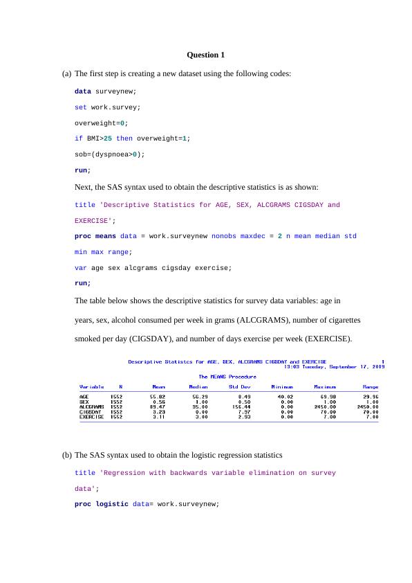
The table below shows the descriptive statistics for survey data variables: age in
years, sex, alcohol consumed per week in grams (ALCGRAMS), number of cigarettes
smoked per day (CIGSDAY), and number of days exercise per week (EXERCISE).
(b) The SAS syntax used to obtain the logistic regression statistics
title 'Regression with backwards variable elimination on survey
data';
proc logistic data= work.surveynew;
(a) The first step is creating a new dataset using the following codes:
data surveynew;
set work.survey;
overweight=0;
if BMI>25 then overweight=1;
sob=(dyspnoea>0);
run;
Next, the SAS syntax used to obtain the descriptive statistics is as shown:
title 'Descriptive Statistics for AGE, SEX, ALCGRAMS CIGSDAY and
EXERCISE';
proc means data = work.surveynew nonobs maxdec = 2 n mean median std
min max range;
var age sex alcgrams cigsday exercise;
run;
The table below shows the descriptive statistics for survey data variables: age in
years, sex, alcohol consumed per week in grams (ALCGRAMS), number of cigarettes
smoked per day (CIGSDAY), and number of days exercise per week (EXERCISE).
(b) The SAS syntax used to obtain the logistic regression statistics
title 'Regression with backwards variable elimination on survey
data';
proc logistic data= work.surveynew;
model overweight(event='1') = age sex alcgrams cigsday exercise
age*sex alcgrams*sex cigsday*sex exercise*sex
/ selection = backward
Slentry = 0.3
Slstay = 0.05
details
lackfit;
run;
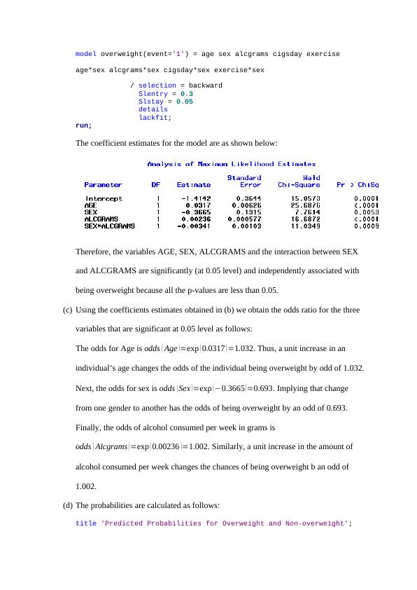
The coefficient estimates for the model are as shown below:
Therefore, the variables AGE, SEX, ALCGRAMS and the interaction between SEX
and ALCGRAMS are significantly (at 0.05 level) and independently associated with
being overweight because all the p-values are less than 0.05.
(c) Using the coefficients estimates obtained in (b) we obtain the odds ratio for the three
variables that are significant at 0.05 level as follows:
The odds for Age is odds ( Age )=exp ( 0.0317 ) =1.032. Thus, a unit increase in an
individual’s age changes the odds of the individual being overweight by odd of 1.032.
Next, the odds for sex is odds ( Sex )=exp (−0.3665 )=0.693. Implying that change
from one gender to another has the odds of being overweight by an odd of 0.693.
Finally, the odds of alcohol consumed per week in grams is
odds ( Alcgrams )=exp ( 0.00236 )=1.002. Similarly, a unit increase in the amount of
alcohol consumed per week changes the chances of being overweight b an odd of
1.002.
(d) The probabilities are calculated as follows:
title 'Predicted Probabilities for Overweight and Non-overweight';
age*sex alcgrams*sex cigsday*sex exercise*sex
/ selection = backward
Slentry = 0.3
Slstay = 0.05
details
lackfit;
run;
The coefficient estimates for the model are as shown below:
Therefore, the variables AGE, SEX, ALCGRAMS and the interaction between SEX
and ALCGRAMS are significantly (at 0.05 level) and independently associated with
being overweight because all the p-values are less than 0.05.
(c) Using the coefficients estimates obtained in (b) we obtain the odds ratio for the three
variables that are significant at 0.05 level as follows:
The odds for Age is odds ( Age )=exp ( 0.0317 ) =1.032. Thus, a unit increase in an
individual’s age changes the odds of the individual being overweight by odd of 1.032.
Next, the odds for sex is odds ( Sex )=exp (−0.3665 )=0.693. Implying that change
from one gender to another has the odds of being overweight by an odd of 0.693.
Finally, the odds of alcohol consumed per week in grams is
odds ( Alcgrams )=exp ( 0.00236 )=1.002. Similarly, a unit increase in the amount of
alcohol consumed per week changes the chances of being overweight b an odd of
1.002.
(d) The probabilities are calculated as follows:
title 'Predicted Probabilities for Overweight and Non-overweight';
proc logistic data= work.surveynew;
model overweight(event='1') = age sex alcgrams sex*alcgrams;
output out = pred p = phat predprob=(individual);
run;
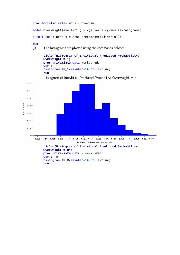
(i) The histograms are plotted using the commands below:
title ‘Histogram of Individual Predicted Probability:
Overweight = 1;
proc univariate data=work.pred;
var IP_1;
histogram IP_1/maxnbin=10 cfill=blue;
run;
title ‘Histogram of Individual Predicted Probability:
Overweight = 0’;
proc univariate data = work.pred;
var IP_0;
histogram IP_0/maxnbin=10 cfill=blue;
run;
model overweight(event='1') = age sex alcgrams sex*alcgrams;
output out = pred p = phat predprob=(individual);
run;
(i) The histograms are plotted using the commands below:
title ‘Histogram of Individual Predicted Probability:
Overweight = 1;
proc univariate data=work.pred;
var IP_1;
histogram IP_1/maxnbin=10 cfill=blue;
run;
title ‘Histogram of Individual Predicted Probability:
Overweight = 0’;
proc univariate data = work.pred;
var IP_0;
histogram IP_0/maxnbin=10 cfill=blue;
run;
End of preview
Want to access all the pages? Upload your documents or become a member.
Related Documents
1. Executive Summary Objective To examine the factors tlg...
|23
|5105
|51