Queuing Theory and Optimization for Traffic Network | Desklib

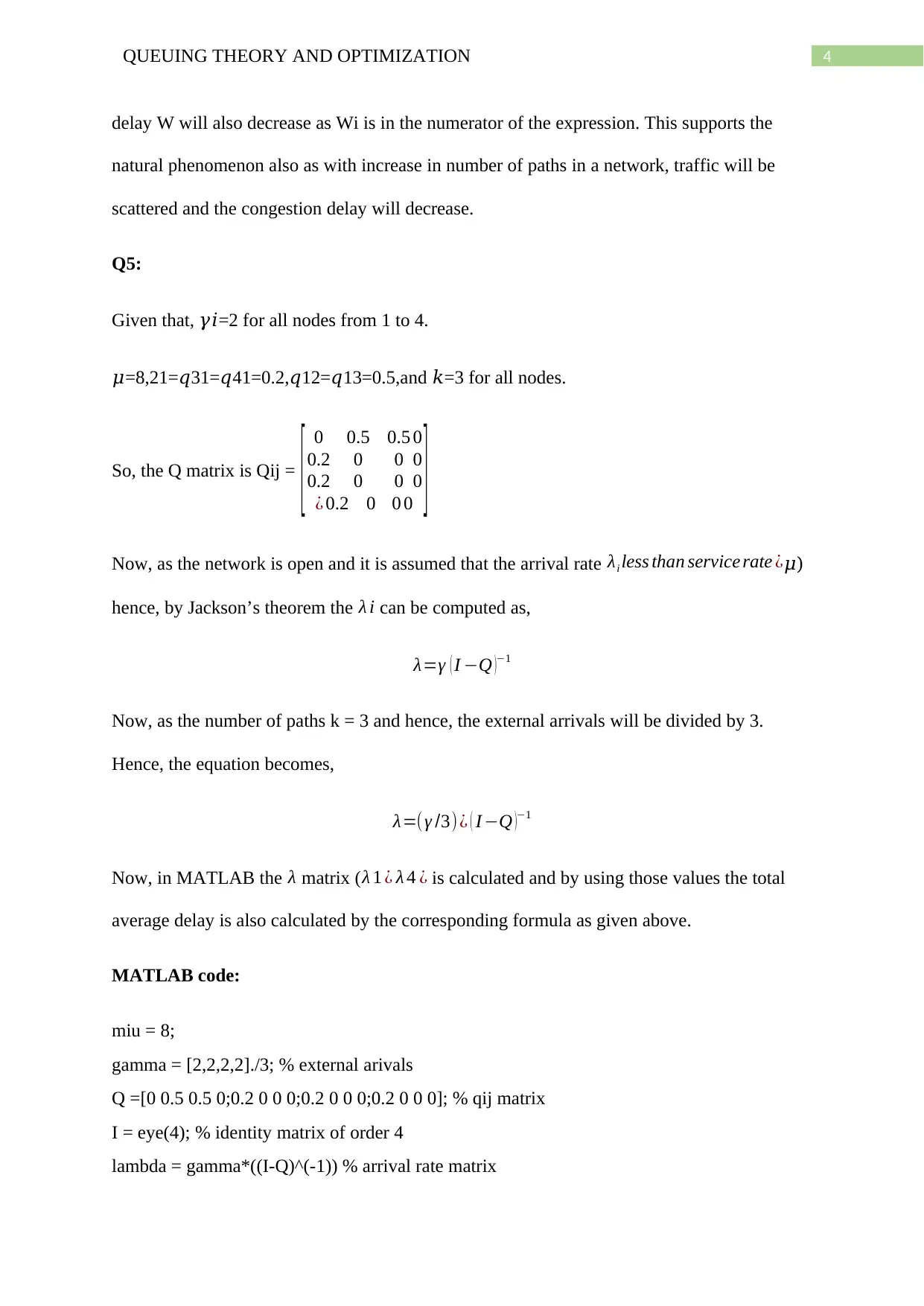
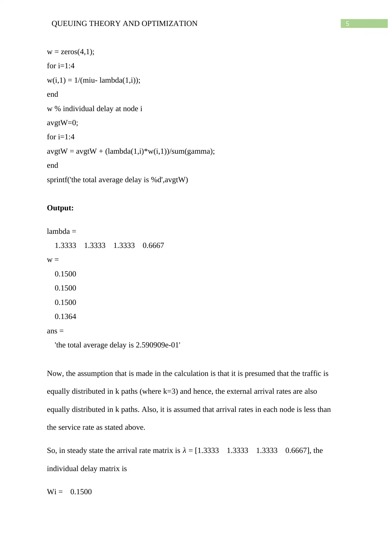
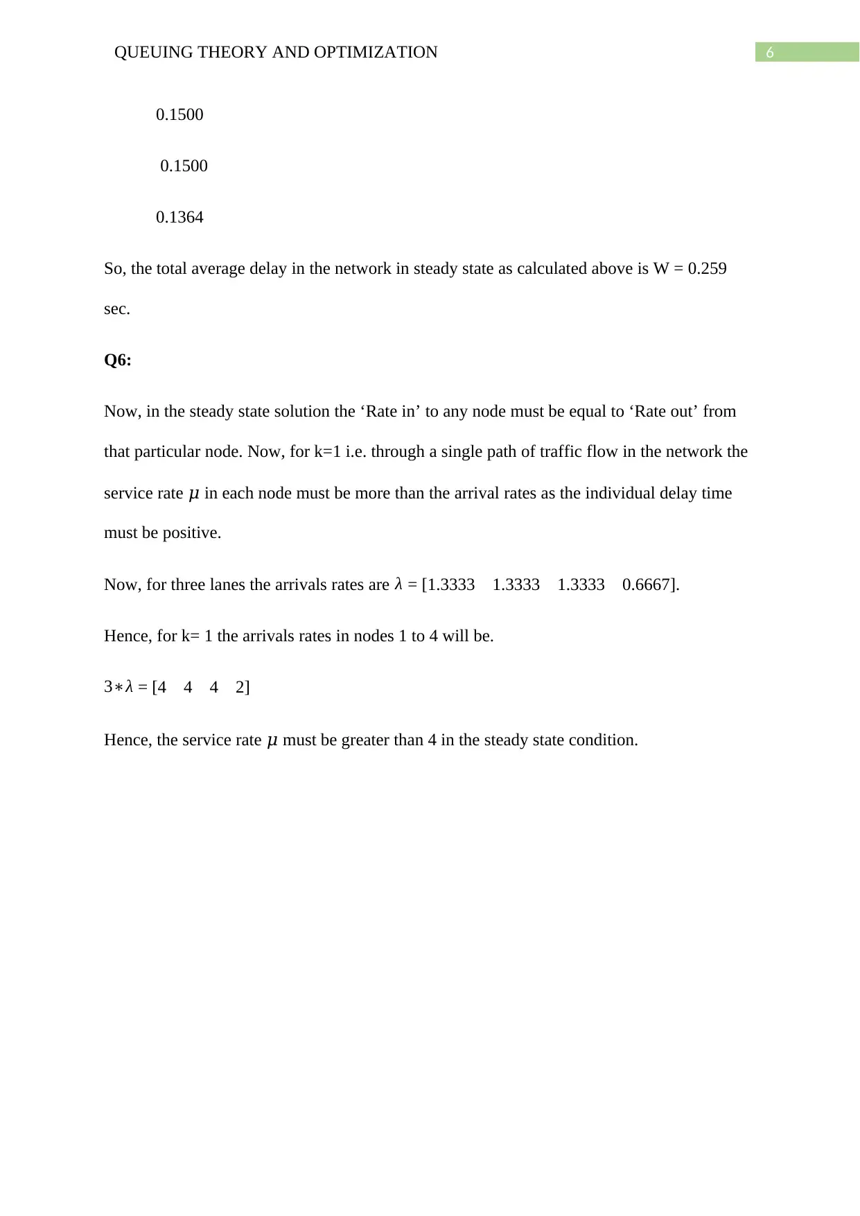
This article discusses Queuing Theory and Optimization for Traffic Network. It covers topics like Jackson queuing network, arrival rate, individual delays, total average delay, steady state solution, and service rate. The article also includes MATLAB code for calculating the arrival rate matrix and individual delay matrix. Subject: Queuing Theory, Course Code: NA, Course Name: NA, College/University: NA

Running head: QUEUING THEORY AND OPTIMIZATION
QUEUING THEORY AND OPTIMIZATION
Name of the Student
Name of the University
Author Note

1QUEUING THEORY AND OPTIMIZATION
The traffic queuing network as given in the question is the following.
Q1:
Now, the Jackson queuing network of the above street network is constructed as follows.
Every line contains k number of paths in the picture given below i.e. traffic enters of leaves
the nodes by k number of paths.

2QUEUING THEORY AND OPTIMIZATION
Q2:
The arrival rate in any Jackson network is given by,
λi=γ i+∑
j =1
4
λ j∗q ji
Hence, the arrival rate at different nodes are
λ1=γ 1+ λ1∗q11+ λ2∗q21+ λ3∗q31 + λ4∗q41
Now, as there is no self-loop in node 1 so q11=0

3QUEUING THEORY AND OPTIMIZATION
So, the expression of λ1 becomes
λ1=γ 1+ λ2∗q21+ λ3∗q31 + λ4∗q41
Similarly, the other equations are
λ2=γ 2+ λ1∗q12+ λ3∗q32 + λ4∗q42
λ3=γ 3 + λ1∗q13 + λ2∗q23 + λ4∗q43
λ4=γ 4 + λ1∗q14 +λ2∗q24+ λ3∗q34
Q3:
The expression of individual delays Wi is given by,
Wi= 1
μi−λi
Where, μi = service rate of the ith node = μ for all the nodes in this case.
λi=¿ Arrival rate at the ith node (for all i=1(1)4).
Now, the total average delay of the network is given by,
W = ∑
i=1
4
( λi
γN ¿)Wi ¿
Where, γN=¿ ∑
i=1
4
γi
Q4:
Now, the above expression of W = ∑
i=1
4
( λi
γN ¿)Wi ¿is for M/M/1 network where the number of
paths or lanes is 1 and as the number of paths are increased it can be seen from the equation
the individual delays Wi will decrease as the service rate μ increases and the total average

4QUEUING THEORY AND OPTIMIZATION
delay W will also decrease as Wi is in the numerator of the expression. This supports the
natural phenomenon also as with increase in number of paths in a network, traffic will be
scattered and the congestion delay will decrease.
Q5:
Given that, 𝛾𝑖=2 for all nodes from 1 to 4.
𝜇=8,21=𝑞31=𝑞41=0.2,𝑞12=𝑞13=0.5,and 𝑘=3 for all nodes.
So, the Q matrix is Qij =
[ 0 0.5 0.5
0.2 0 0
0.2 0 0
0
0
0
¿ 0.2 0 0 0 ]
Now, as the network is open and it is assumed that the arrival rate λi less than service rate ¿𝜇)
hence, by Jackson’s theorem the λ i can be computed as,
λ=γ ( I −Q )−1
Now, as the number of paths k = 3 and hence, the external arrivals will be divided by 3.
Hence, the equation becomes,
λ=(γ /3) ¿ ( I −Q )−1
Now, in MATLAB the λ matrix ( λ 1 ¿ λ 4 ¿ is calculated and by using those values the total
average delay is also calculated by the corresponding formula as given above.
MATLAB code:
miu = 8;
gamma = [2,2,2,2]./3; % external arivals
Q =[0 0.5 0.5 0;0.2 0 0 0;0.2 0 0 0;0.2 0 0 0]; % qij matrix
I = eye(4); % identity matrix of order 4
lambda = gamma*((I-Q)^(-1)) % arrival rate matrix

5QUEUING THEORY AND OPTIMIZATION
w = zeros(4,1);
for i=1:4
w(i,1) = 1/(miu- lambda(1,i));
end
w % individual delay at node i
avgtW=0;
for i=1:4
avgtW = avgtW + (lambda(1,i)*w(i,1))/sum(gamma);
end
sprintf('the total average delay is %d',avgtW)
Output:
lambda =
1.3333 1.3333 1.3333 0.6667
w =
0.1500
0.1500
0.1500
0.1364
ans =
'the total average delay is 2.590909e-01'
Now, the assumption that is made in the calculation is that it is presumed that the traffic is
equally distributed in k paths (where k=3) and hence, the external arrival rates are also
equally distributed in k paths. Also, it is assumed that arrival rates in each node is less than
the service rate as stated above.
So, in steady state the arrival rate matrix is λ = [1.3333 1.3333 1.3333 0.6667], the
individual delay matrix is
Wi = 0.1500

6QUEUING THEORY AND OPTIMIZATION
0.1500
0.1500
0.1364
So, the total average delay in the network in steady state as calculated above is W = 0.259
sec.
Q6:
Now, in the steady state solution the ‘Rate in’ to any node must be equal to ‘Rate out’ from
that particular node. Now, for k=1 i.e. through a single path of traffic flow in the network the
service rate 𝜇 in each node must be more than the arrival rates as the individual delay time
must be positive.
Now, for three lanes the arrivals rates are λ = [1.3333 1.3333 1.3333 0.6667].
Hence, for k= 1 the arrivals rates in nodes 1 to 4 will be.
3∗λ = [4 4 4 2]
Hence, the service rate 𝜇 must be greater than 4 in the steady state condition.