Economics Assignment: Zero-Coupon Bonds, Demand Curves, and Analysis

This finance assignment analyzes the behavior of interest rates and the models used to predict them, focusing on zero-coupon bonds. The assignment explores the calculation of expected returns for a one-year, $1000 face value bond at different market prices, revealing the relationship between market price and return. It then delves into market equilibrium, explaining how supply and demand interact to determine bond prices and interest rates, and uses the expected return formula to demonstrate this relationship. Finally, the assignment examines factors that shift the demand curve (wealth increment, decline in expected return) and supply curve (increase in inflation, government borrowing), illustrating each factor with diagrams and real-world examples to connect theory with practice. The analysis covers various economic concepts and their impact on the bond market, providing insights into investment strategies and market dynamics.

qwertyuiopasdfghjklzxcvbnmqwertyui
opasdfghjklzxcvbnmqwertyuiopasdfgh
jklzxcvbnmqwertyuiopasdfghjklzxcvb
nmqwertyuiopasdfghjklzxcvbnmqwer
tyuiopasdfghjklzxcvbnmqwertyuiopas
dfghjklzxcvbnmqwertyuiopasdfghjklzx
cvbnmqwertyuiopasdfghjklzxcvbnmq
wertyuiopasdfghjklzxcvbnmqwertyuio
pasdfghjklzxcvbnmqwertyuiopasdfghj
klzxcvbnmqwertyuiopasdfghjklzxcvbn
mqwertyuiopasdfghjklzxcvbnmqwerty
uiopasdfghjklzxcvbnmqwertyuiopasdf
ghjklzxcvbnmqwertyuiopasdfghjklzxc
vbnmqwertyuiopasdfghjklzxcvbnmrty
uiopasdfghjklzxcvbnmqwertyuiopasdf
ghjklzxcvbnmqwertyuiopasdfghjklzxc
Investment Analysis and Portfolio Management

Economics
Answer – 1
There are some bonds that are issued in order to provide a discount on the face value of the
bonds, still, there are no visible interest rates observed on them. The interest acquired on these
bonds is referred to a coupon. These bonds are also called zero-coupon bonds because of the zero
dividends or interest rate they provided. These bonds are bought at the market value and after
their maturity; they are repaid at their face value (Deegan, 2011). The difference between the
amount of market value and face value is termed to be a coupon. For this particular assignment,
there are 4 major bonds that are needed to be analyzed and computed. All the bonds can be
understood with the help of an example. The bonds will be held for 1 year because of which time
will not be a factor while making the comparison. Expected return rate if the market price of the
bond is $800.
A. The face value of a given zero coupon bond is stated to be $1000. The time period and in
which it will mature is one year.
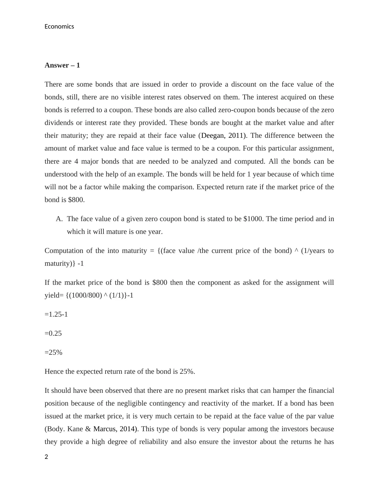
Computation of the into maturity = {(face value /the current price of the bond) ^ (1/years to
maturity)} -1
If the market price of the bond is $800 then the component as asked for the assignment will
yield= {(1000/800) ^ (1/1)}-1
=1.25-1
=0.25
=25%
Hence the expected return rate of the bond is 25%.
It should have been observed that there are no present market risks that can hamper the financial
position because of the negligible contingency and reactivity of the market. If a bond has been
issued at the market price, it is very much certain to be repaid at the face value of the par value
(Body. Kane & Marcus, 2014). This type of bonds is very popular among the investors because
they provide a high degree of reliability and also ensure the investor about the returns he has
2

Economics
received from their investment at the end of the bond period. The zero coupon bonds are also
said to act as market thresholds because the rate fluctuate based on the zero coupon bond rates as
well. These bonds are also said to be volatile in nature because of which they do not offer any
kind of fixed return rate in a given period of time and also the yield depends on the bond types
and issuers (Titman, Martin, Keown & Martin, 2016).
The bond which yields 25% will be greater than the interest rates that are provided by most of
the other investment opportunities because of which demand of the bond will exceed the supply.
Increase in the interest rate of the market will be observed and inflationary tendencies in the
economy can also be noticed.
B. The expected return of the market rate of the bond is $950.
The given face value of a zero coupon bond is $1000. The time to maturity is 1 year.
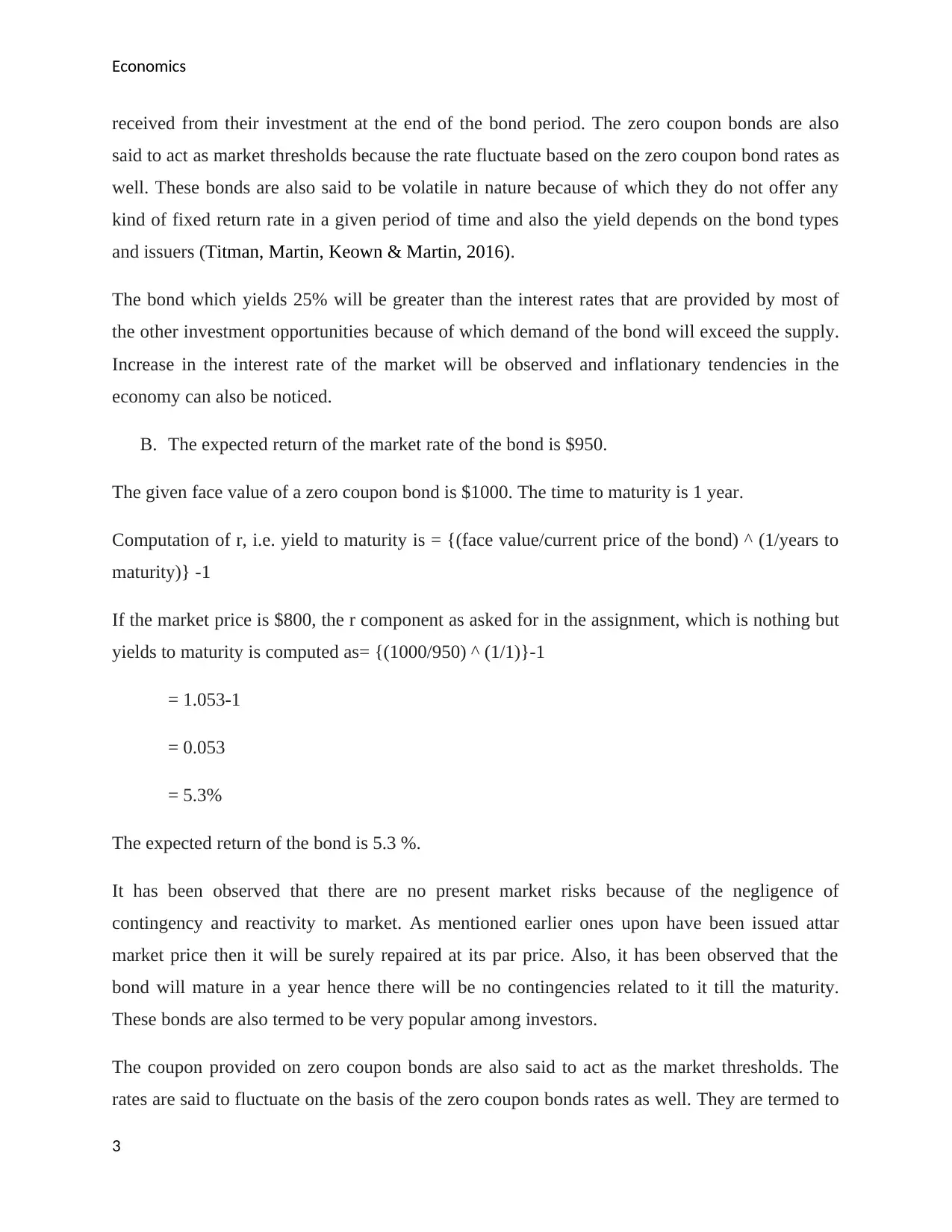
Computation of r, i.e. yield to maturity is = {(face value/current price of the bond) ^ (1/years to
maturity)} -1
If the market price is $800, the r component as asked for in the assignment, which is nothing but
yields to maturity is computed as= {(1000/950) ^ (1/1)}-1
= 1.053-1
= 0.053
= 5.3%
The expected return of the bond is 5.3 %.
It has been observed that there are no present market risks because of the negligence of
contingency and reactivity to market. As mentioned earlier ones upon have been issued attar
market price then it will be surely repaired at its par price. Also, it has been observed that the
bond will mature in a year hence there will be no contingencies related to it till the maturity.
These bonds are also termed to be very popular among investors.
The coupon provided on zero coupon bonds are also said to act as the market thresholds. The
rates are said to fluctuate on the basis of the zero coupon bonds rates as well. They are termed to
3

Economics
be volatile because they do not offer any kind of eggs return rate during a given period of time.
Hence the yield on the bonds is subjective to the bind types and issuers. The market will be said
to have an equilibrium position because the bond yield will be the same as most of the interest
rates.
The expected return of the market price of the bond is $1000.
The face value of a given zero coupon bond is $1,000 and the time to maturity is one year
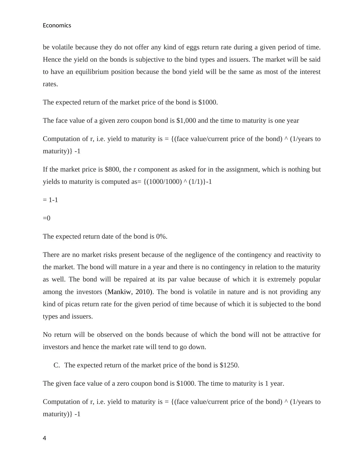
Computation of r, i.e. yield to maturity is = {(face value/current price of the bond) ^ (1/years to
maturity)} -1
If the market price is $800, the r component as asked for in the assignment, which is nothing but
yields to maturity is computed as= {(1000/1000) ^ (1/1)}-1
= 1-1
=0
The expected return date of the bond is 0%.
There are no market risks present because of the negligence of the contingency and reactivity to
the market. The bond will mature in a year and there is no contingency in relation to the maturity
as well. The bond will be repaired at its par value because of which it is extremely popular
among the investors (Mankiw, 2010). The bond is volatile in nature and is not providing any
kind of picas return rate for the given period of time because of which it is subjected to the bond
types and issuers.
No return will be observed on the bonds because of which the bond will not be attractive for
investors and hence the market rate will tend to go down.
C. The expected return of the market price of the bond is $1250.
The given face value of a zero coupon bond is $1000. The time to maturity is 1 year.
Computation of r, i.e. yield to maturity is = {(face value/current price of the bond) ^ (1/years to
maturity)} -1
4

Economics
If the market price is $800, the r component as asked for in the assignment, which is nothing but
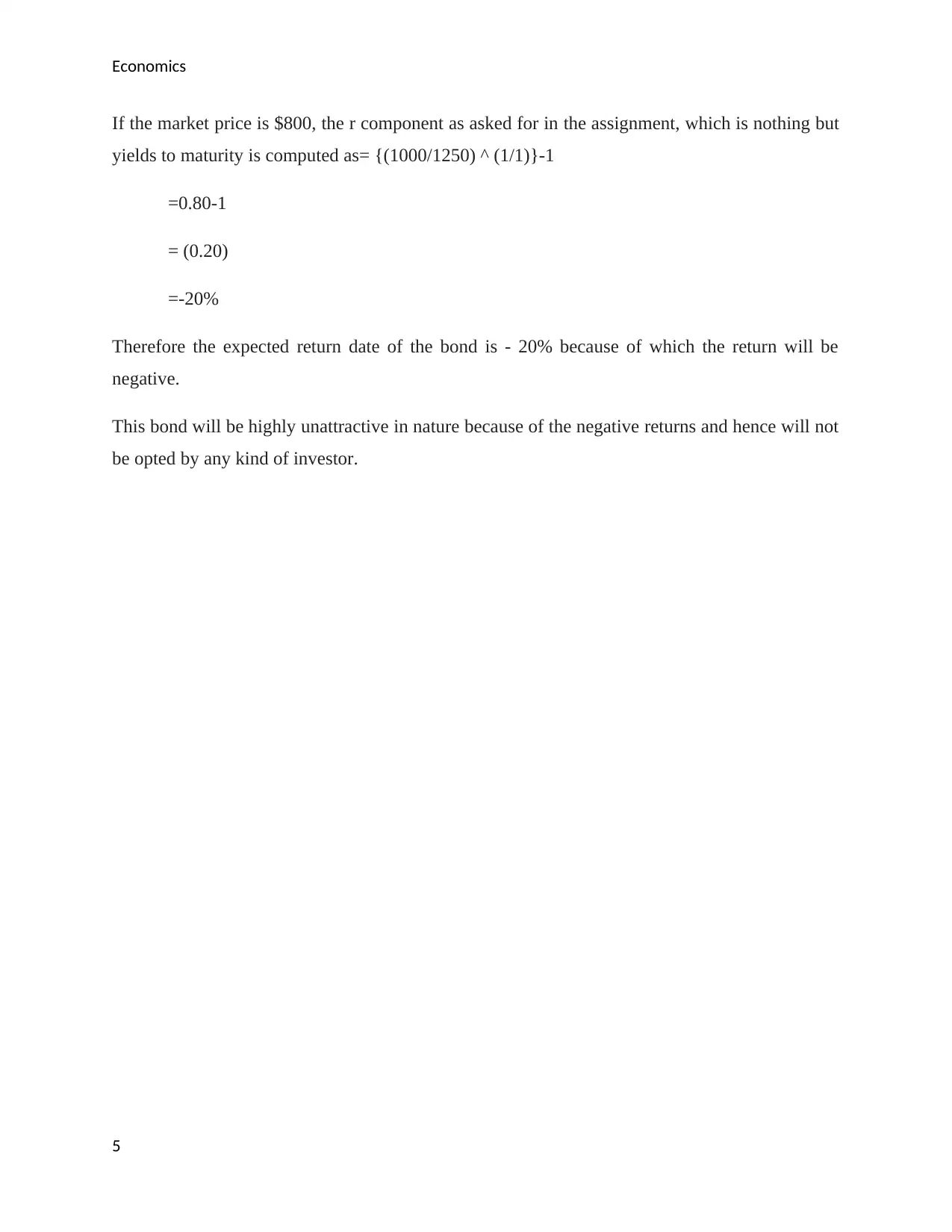
yields to maturity is computed as= {(1000/1250) ^ (1/1)}-1
=0.80-1
= (0.20)
=-20%
Therefore the expected return date of the bond is - 20% because of which the return will be
negative.
This bond will be highly unattractive in nature because of the negative returns and hence will not
be opted by any kind of investor.
5

Economics
Answer – 2
Expected return can be said to be the mechanism that enables the determination of investment
into positive or negative net income into an average basis. The computation is done in terms of
the investment expected value and is done considering various scenarios (Berk, DeMarzo &
Stangeland, 2015). Expected return can be said to be the return that in predicted or the budgeted
gain on the zero coupon bonds. In this scenario, we are dealing with the investment that is zero
coupons where the face value stands at $1000 and the period of maturity stands at one year.
The computation of the expected return is done by the following formula:
E= (F-M)/M
Here E pertains to the return that is expected, F denotes the face value while M stands for market
value.
i) In this case where M = $800
E = (1000-800)/800
=25%
ii) Scenario where M= $950
E= (1000-950)/950
=5.26%
iii) Scenario where M = $1000
iv) When M= $1000
E= (1000-1000)/1000
=0
v) When M= $1250
6

Economics
E= (1000-1250)/1250
= -20%
It is observed that an increment in the market prices from $800 to $950 and ultimately $1250,
there is a decline in the expected returns. This provides a clarification that when the price gap
stands huge between the market price and the FV, the expected return is higher in nature. The
difference between the price gap ascertains the return that is expected.
However, it needs to be noted that other model can be utilized in this scenario to forecst the
rate of interest like the variance model, the SD model, etc. In the case of variance model, the
calculation of the expected value is done for sale and the difference is squared. Finally the
weighted average is calculated to know the variance (Mankiw Gregoryand and William,
2011). The same variance when utilized on a portfolio becomes a portfolio variance.
Standard deviation is computed by knowing the square root of the variance. This leads to the
model of the standard deviation (Petty, Titman, Keown, Martin, Burrow, Nguyen, 2012).
Expected rate of return = 20%
FV = $1000
As per the formula,
E= (F-M)/M
The given expected rate of return = 20%.
Face value = $1000
Here, E is return that is expected, F denotes FV and M is the MV
Hence,
0.2= (1000-M)/M
0.2M + M = 1000
1.2M=1000
7

Economics
M= 833.33
From the above situation it can be seen that higher expected rate of return means more gap
between the FV and the MV. When the market price is less than the FV and MV difference than
investors will have high level of profit while in case of market price is more than the FV then
expected return will be less than zero (Madura & Fox, 2011). When the negative expected rate of
return happens then the investor will face losses in terms of investment and the return. Thereby,
negative return leads to losses and destructs the investment (Peirson, Brown, Easton, Howard, &
Pinder, 2015)
8

Economics
Answer 3
Shift in the curves
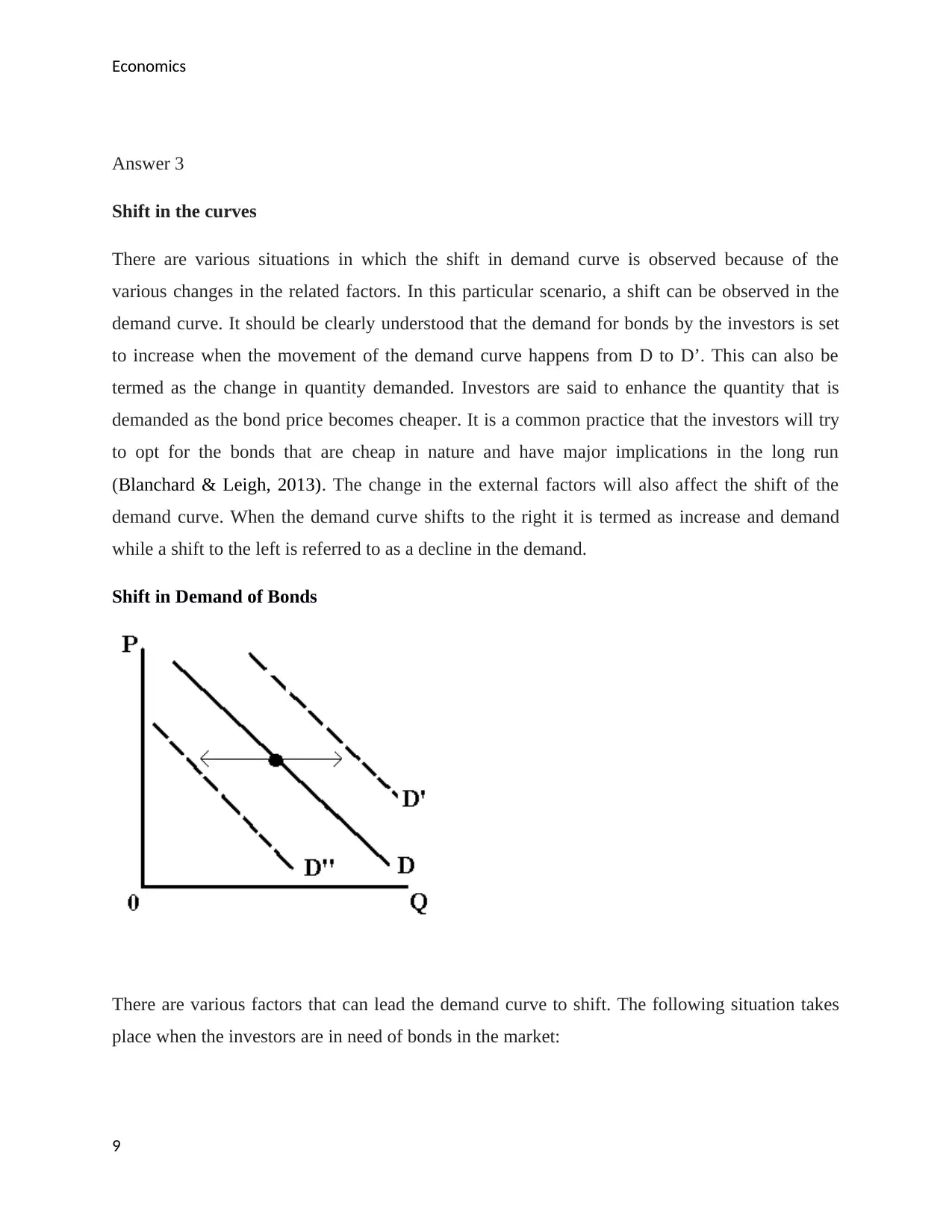
There are various situations in which the shift in demand curve is observed because of the
various changes in the related factors. In this particular scenario, a shift can be observed in the
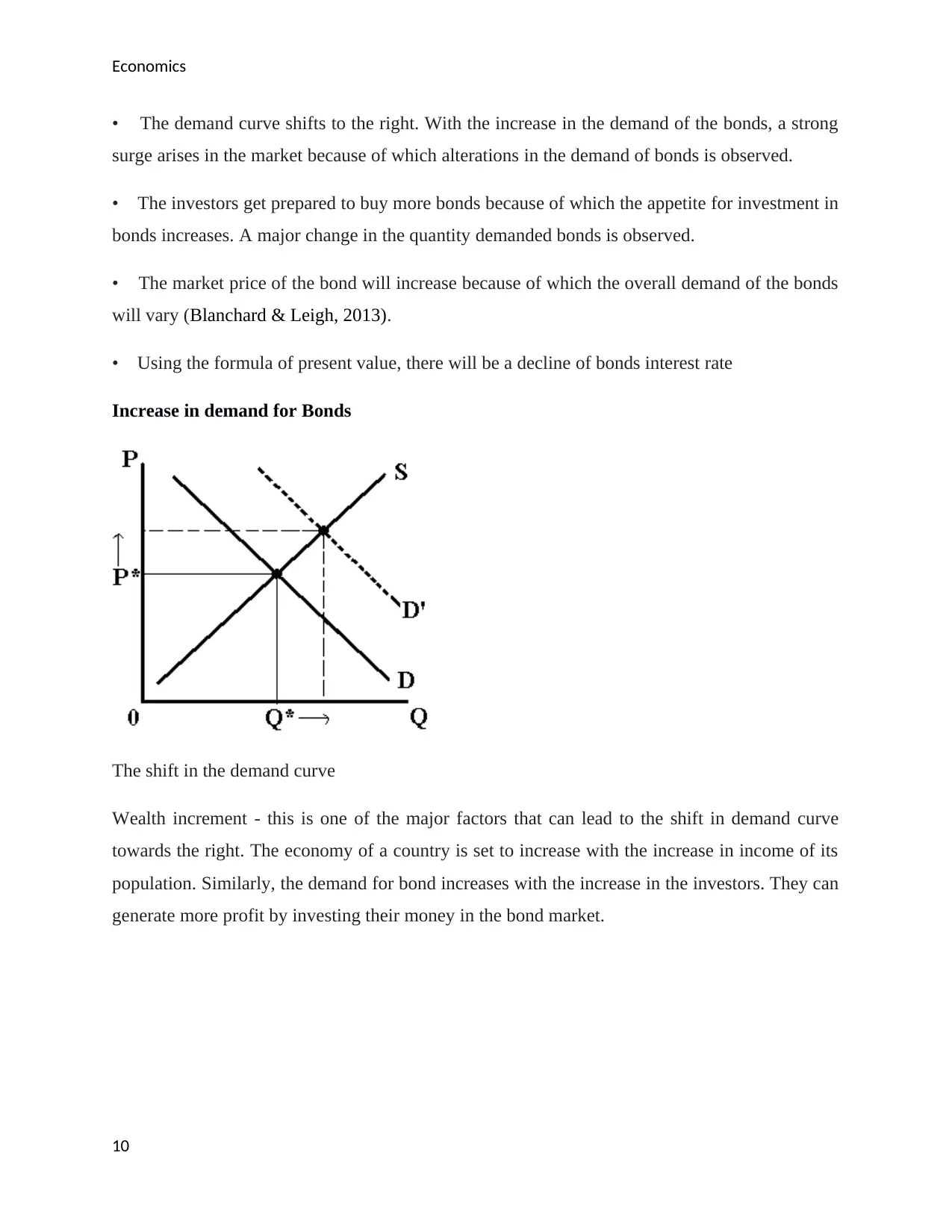
demand curve. It should be clearly understood that the demand for bonds by the investors is set
to increase when the movement of the demand curve happens from D to D’. This can also be
termed as the change in quantity demanded. Investors are said to enhance the quantity that is
demanded as the bond price becomes cheaper. It is a common practice that the investors will try
to opt for the bonds that are cheap in nature and have major implications in the long run
(Blanchard & Leigh, 2013). The change in the external factors will also affect the shift of the
demand curve. When the demand curve shifts to the right it is termed as increase and demand
while a shift to the left is referred to as a decline in the demand.
Shift in Demand of Bonds
There are various factors that can lead the demand curve to shift. The following situation takes
place when the investors are in need of bonds in the market:
9

Economics
• The demand curve shifts to the right. With the increase in the demand of the bonds, a strong
surge arises in the market because of which alterations in the demand of bonds is observed.
• The investors get prepared to buy more bonds because of which the appetite for investment in
bonds increases. A major change in the quantity demanded bonds is observed.
• The market price of the bond will increase because of which the overall demand of the bonds
will vary (Blanchard & Leigh, 2013).
• Using the formula of present value, there will be a decline of bonds interest rate
Increase in demand for Bonds
The shift in the demand curve
Wealth increment - this is one of the major factors that can lead to the shift in demand curve
towards the right. The economy of a country is set to increase with the increase in income of its
population. Similarly, the demand for bond increases with the increase in the investors. They can
generate more profit by investing their money in the bond market.
10

Economics
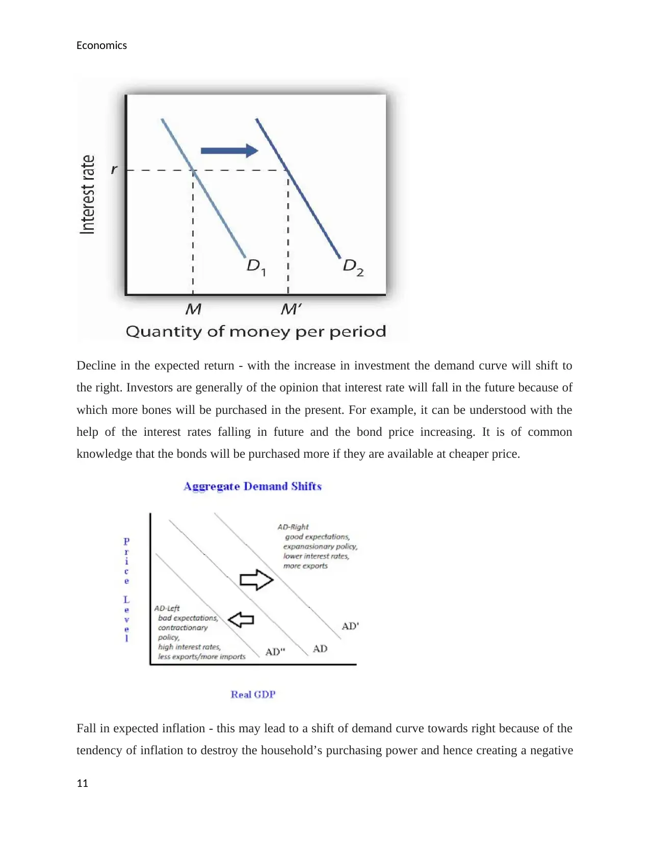
Decline in the expected return - with the increase in investment the demand curve will shift to
the right. Investors are generally of the opinion that interest rate will fall in the future because of
which more bones will be purchased in the present. For example, it can be understood with the
help of the interest rates falling in future and the bond price increasing. It is of common
knowledge that the bonds will be purchased more if they are available at cheaper price.
Fall in expected inflation - this may lead to a shift of demand curve towards right because of the
tendency of inflation to destroy the household’s purchasing power and hence creating a negative
11

Economics
impact on the government and businesses. The value of the investments can observe a major fall
and hence it is needed to be noted that the investments made by the investors will observe and an
inflation rate that will increase specifically in relation to the bonds (Amadeo, 2011). However, if
the investors will observe stability in the market then they will buy more bonds.
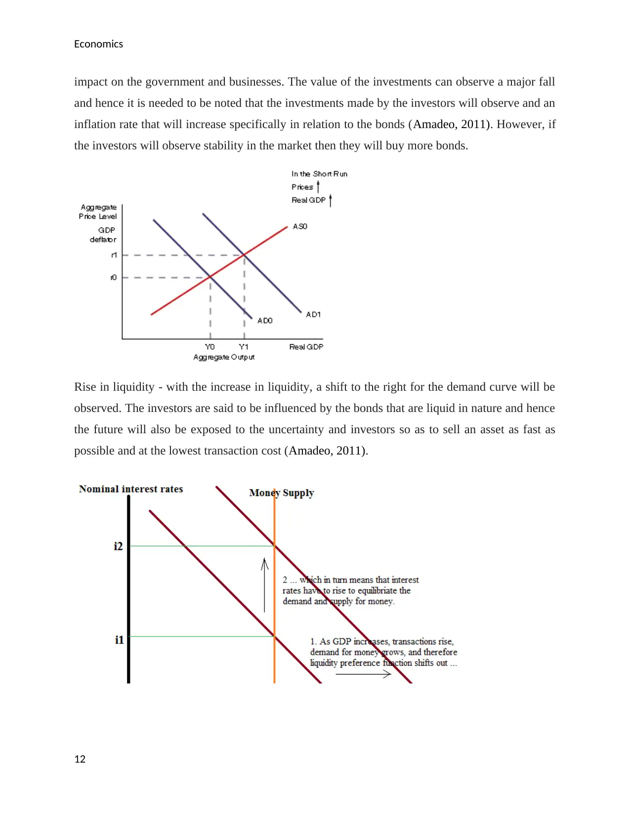
Rise in liquidity - with the increase in liquidity, a shift to the right for the demand curve will be
observed. The investors are said to be influenced by the bonds that are liquid in nature and hence
the future will also be exposed to the uncertainty and investors so as to sell an asset as fast as
possible and at the lowest transaction cost (Amadeo, 2011).
12