R Programming Analysis 2022
VerifiedAdded on 2022/09/12
|7
|1725
|21
AI Summary
Contribute Materials
Your contribution can guide someone’s learning journey. Share your
documents today.
R Programming 1
R Programming
(Name of Student)
(Institutional Affiliation)
(Date of Submission)
R Programming
(Name of Student)
(Institutional Affiliation)
(Date of Submission)
Secure Best Marks with AI Grader
Need help grading? Try our AI Grader for instant feedback on your assignments.
R Programming 2
I. Exploratory Data Analysis (EDA)
Directions:
1. Using the provided dataset, do the following:
a. Choose four (4) predictors you feel are the most important and produce scatter plots of the
response variable vs. these predictors.
The following predictors are chosen
b. For each plot, put the response variable on the y-axis and the predictor on the x-axis.
c. Write up one (1) sentence to explain each scatter plot.
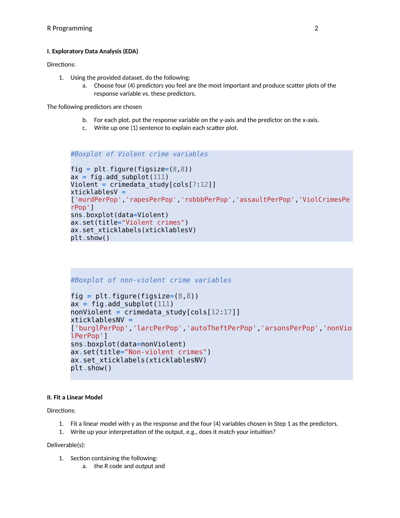
#Boxplot of Violent crime variables
fig = plt.figure(figsize=(8,8))
ax = fig.add_subplot(111)
Violent = crimedata_study[cols[7:12]]
xticklablesV =
['murdPerPop','rapesPerPop','robbbPerPop','assaultPerPop','ViolCrimesPe
rPop']
sns.boxplot(data=Violent)
ax.set(title="Violent crimes")
ax.set_xticklabels(xticklablesV)
plt.show()
#Boxplot of non-violent crime variables
fig = plt.figure(figsize=(8,8))
ax = fig.add_subplot(111)
nonViolent = crimedata_study[cols[12:17]]
xticklablesNV =
['burglPerPop','larcPerPop','autoTheftPerPop','arsonsPerPop','nonVio
lPerPop']
sns.boxplot(data=nonViolent)
ax.set(title="Non-violent crimes")
ax.set_xticklabels(xticklablesNV)
plt.show()
II. Fit a Linear Model
Directions:
1. Fit a linear model with y as the response and the four (4) variables chosen in Step 1 as the predictors.
1. Write up your interpretation of the output, e.g., does it match your intuition?
Deliverable(s):
1. Section containing the following:
a. the R code and output and
I. Exploratory Data Analysis (EDA)
Directions:
1. Using the provided dataset, do the following:
a. Choose four (4) predictors you feel are the most important and produce scatter plots of the
response variable vs. these predictors.
The following predictors are chosen
b. For each plot, put the response variable on the y-axis and the predictor on the x-axis.
c. Write up one (1) sentence to explain each scatter plot.
#Boxplot of Violent crime variables
fig = plt.figure(figsize=(8,8))
ax = fig.add_subplot(111)
Violent = crimedata_study[cols[7:12]]
xticklablesV =
['murdPerPop','rapesPerPop','robbbPerPop','assaultPerPop','ViolCrimesPe
rPop']
sns.boxplot(data=Violent)
ax.set(title="Violent crimes")
ax.set_xticklabels(xticklablesV)
plt.show()
#Boxplot of non-violent crime variables
fig = plt.figure(figsize=(8,8))
ax = fig.add_subplot(111)
nonViolent = crimedata_study[cols[12:17]]
xticklablesNV =
['burglPerPop','larcPerPop','autoTheftPerPop','arsonsPerPop','nonVio
lPerPop']
sns.boxplot(data=nonViolent)
ax.set(title="Non-violent crimes")
ax.set_xticklabels(xticklablesNV)
plt.show()
II. Fit a Linear Model
Directions:
1. Fit a linear model with y as the response and the four (4) variables chosen in Step 1 as the predictors.
1. Write up your interpretation of the output, e.g., does it match your intuition?
Deliverable(s):
1. Section containing the following:
a. the R code and output and
R Programming 3
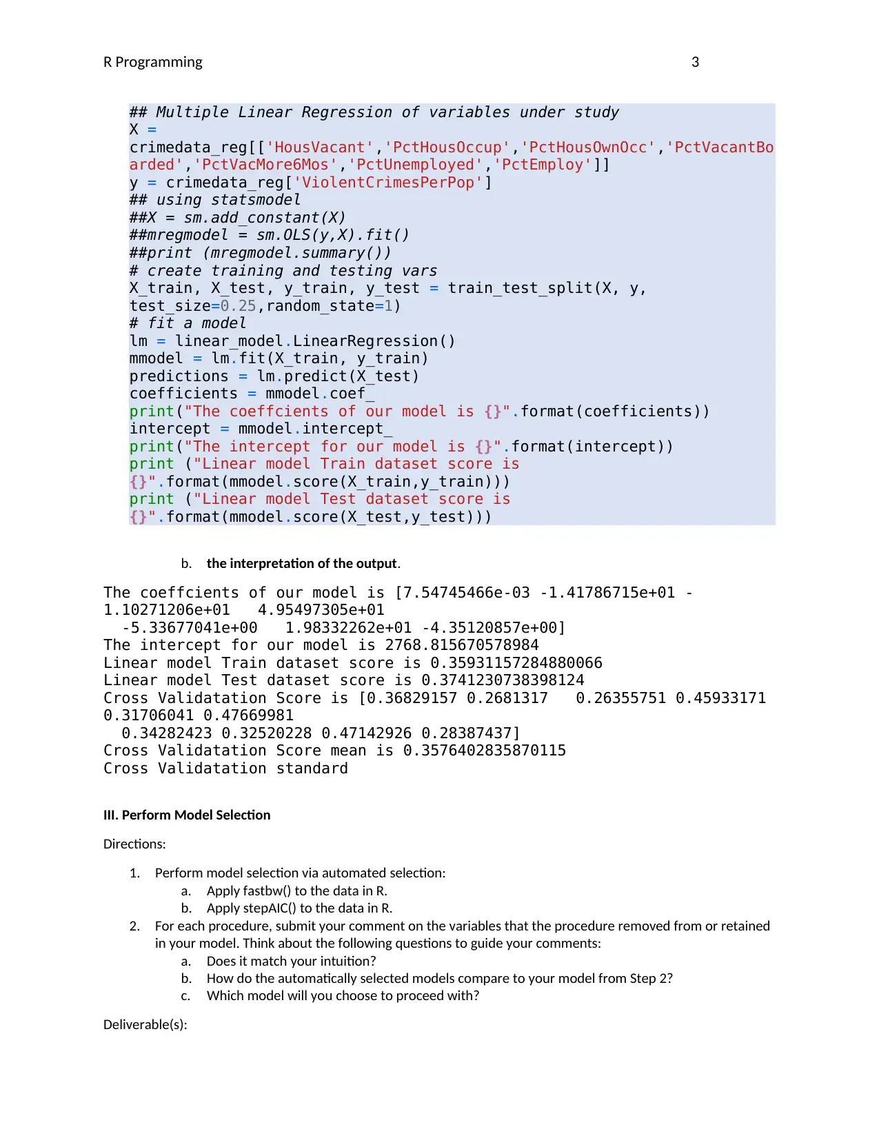
## Multiple Linear Regression of variables under study
X =
crimedata_reg[['HousVacant','PctHousOccup','PctHousOwnOcc','PctVacantBo
arded','PctVacMore6Mos','PctUnemployed','PctEmploy']]
y = crimedata_reg['ViolentCrimesPerPop']
## using statsmodel
##X = sm.add_constant(X)
##mregmodel = sm.OLS(y,X).fit()
##print (mregmodel.summary())
# create training and testing vars
X_train, X_test, y_train, y_test = train_test_split(X, y,
test_size=0.25,random_state=1)
# fit a model
lm = linear_model.LinearRegression()
mmodel = lm.fit(X_train, y_train)
predictions = lm.predict(X_test)
coefficients = mmodel.coef_
print("The coeffcients of our model is {}".format(coefficients))
intercept = mmodel.intercept_
print("The intercept for our model is {}".format(intercept))
print ("Linear model Train dataset score is
{}".format(mmodel.score(X_train,y_train)))
print ("Linear model Test dataset score is
{}".format(mmodel.score(X_test,y_test)))
b. the interpretation of the output.
The coeffcients of our model is [7.54745466e-03 -1.41786715e+01 -
1.10271206e+01 4.95497305e+01
-5.33677041e+00 1.98332262e+01 -4.35120857e+00]
The intercept for our model is 2768.815670578984
Linear model Train dataset score is 0.35931157284880066
Linear model Test dataset score is 0.3741230738398124
Cross Validatation Score is [0.36829157 0.2681317 0.26355751 0.45933171
0.31706041 0.47669981
0.34282423 0.32520228 0.47142926 0.28387437]
Cross Validatation Score mean is 0.3576402835870115
Cross Validatation standard deviation is 0.07924703838521946
III. Perform Model Selection
Directions:
1. Perform model selection via automated selection:
a. Apply fastbw() to the data in R.
b. Apply stepAIC() to the data in R.
2. For each procedure, submit your comment on the variables that the procedure removed from or retained
in your model. Think about the following questions to guide your comments:
a. Does it match your intuition?
b. How do the automatically selected models compare to your model from Step 2?
c. Which model will you choose to proceed with?
Deliverable(s):
R Programming 4
1. Section containing the following:
a. R code and output and
b. comments on the variables.
IV. Apply Diagnostics to the Model
Directions:
1. Perform diagnostics on the model chosen in Step 3 to check the mathematical assumptions of the model.
2. Produce the following three (3) plots:
a. Fitted values vs. residuals plot.
b. Q-Q plot.
c. Lagged residual plot (i.e., right hand plot in Figure 6.7 in the text).
3. For each, provide one sentence to explain whether they indicate if the model assumptions are upheld. If
the assumptions do not appear to be upheld, then hang tight, as this is addressed in a later step.
Deliverable(s):
1. Section containing the following:
a. the three (3) plots,
b. the associated R code, and
c. explanations of the model assumptions.
V. Investigate Fit for Individual Observations
Directions:
1. Check for outliers and influential observations.
2. Write up brief explanations as to what you are seeing.
Deliverable(s):
1. Section containing the following:
a. the code used to calculate standardized residuals and Cook’s Distance,
b. the code used to identify outliers and influential observations (don’t paste all individual values),
and
c. the brief explanations as to what you are seeing.
VI. Apply Transformations to the Model as Needed
Directions:
1. Correct the model if mathematical assumptions of the model were not met in Step 4.
a. If a transformation is needed, indicate what measures you are taking (i.e., Box-Cox
transformation, polynomial regression, or some method that wasn’t covered if you’re feeling
adventurous).
b. If a transformation is not needed, run the Box-Cox method anyway to see if the result agrees
with your intuitive assessment from Step 4.
Deliverable(s):
1. Section containing the following:
a. Methods used for correcting or applying the transformations listed above.
VII. Report Inferences and Make Predictions Using a Final Model
Directions:
1. Report your final model and use it to perform inferences.
1. Section containing the following:
a. R code and output and
b. comments on the variables.
IV. Apply Diagnostics to the Model
Directions:
1. Perform diagnostics on the model chosen in Step 3 to check the mathematical assumptions of the model.
2. Produce the following three (3) plots:
a. Fitted values vs. residuals plot.
b. Q-Q plot.
c. Lagged residual plot (i.e., right hand plot in Figure 6.7 in the text).
3. For each, provide one sentence to explain whether they indicate if the model assumptions are upheld. If
the assumptions do not appear to be upheld, then hang tight, as this is addressed in a later step.
Deliverable(s):
1. Section containing the following:
a. the three (3) plots,
b. the associated R code, and
c. explanations of the model assumptions.
V. Investigate Fit for Individual Observations
Directions:
1. Check for outliers and influential observations.
2. Write up brief explanations as to what you are seeing.
Deliverable(s):
1. Section containing the following:
a. the code used to calculate standardized residuals and Cook’s Distance,
b. the code used to identify outliers and influential observations (don’t paste all individual values),
and
c. the brief explanations as to what you are seeing.
VI. Apply Transformations to the Model as Needed
Directions:
1. Correct the model if mathematical assumptions of the model were not met in Step 4.
a. If a transformation is needed, indicate what measures you are taking (i.e., Box-Cox
transformation, polynomial regression, or some method that wasn’t covered if you’re feeling
adventurous).
b. If a transformation is not needed, run the Box-Cox method anyway to see if the result agrees
with your intuitive assessment from Step 4.
Deliverable(s):
1. Section containing the following:
a. Methods used for correcting or applying the transformations listed above.
VII. Report Inferences and Make Predictions Using a Final Model
Directions:
1. Report your final model and use it to perform inferences.
Secure Best Marks with AI Grader
Need help grading? Try our AI Grader for instant feedback on your assignments.
R Programming 5
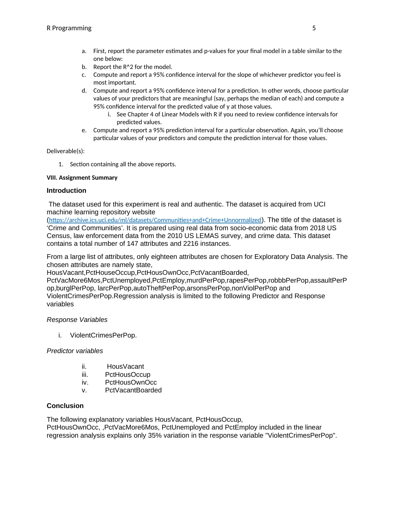
a. First, report the parameter estimates and p-values for your final model in a table similar to the
one below:
b. Report the R^2 for the model.
c. Compute and report a 95% confidence interval for the slope of whichever predictor you feel is
most important.
d. Compute and report a 95% confidence interval for a prediction. In other words, choose particular
values of your predictors that are meaningful (say, perhaps the median of each) and compute a
95% confidence interval for the predicted value of y at those values.
i. See Chapter 4 of Linear Models with R if you need to review confidence intervals for
predicted values.
e. Compute and report a 95% prediction interval for a particular observation. Again, you’ll choose
particular values of your predictors and compute the prediction interval for those values.
Deliverable(s):
1. Section containing all the above reports.
VIII. Assignment Summary
Introduction
The dataset used for this experiment is real and authentic. The dataset is acquired from UCI
machine learning repository website
(https://archive.ics.uci.edu/ml/datasets/Communities+and+Crime+Unnormalized). The title of the dataset is
‘Crime and Communities’. It is prepared using real data from socio-economic data from 2018 US
Census, law enforcement data from the 2010 US LEMAS survey, and crime data. This dataset
contains a total number of 147 attributes and 2216 instances.
From a large list of attributes, only eighteen attributes are chosen for Exploratory Data Analysis. The
chosen attributes are namely state,
HousVacant,PctHouseOccup,PctHousOwnOcc,PctVacantBoarded,
PctVacMore6Mos,PctUnemployed,PctEmploy,murdPerPop,rapesPerPop,robbbPerPop,assaultPerP
op,burglPerPop, larcPerPop,autoTheftPerPop,arsonsPerPop,nonViolPerPop and
ViolentCrimesPerPop.Regression analysis is limited to the following Predictor and Response
variables
Response Variables
i. ViolentCrimesPerPop.
Predictor variables
ii. HousVacant
iii. PctHousOccup
iv. PctHousOwnOcc
v. PctVacantBoarded
Conclusion
The following explanatory variables HousVacant, PctHousOccup,
PctHousOwnOcc, ,PctVacMore6Mos, PctUnemployed and PctEmploy included in the linear
regression analysis explains only 35% variation in the response variable "ViolentCrimesPerPop".
R Programming 6
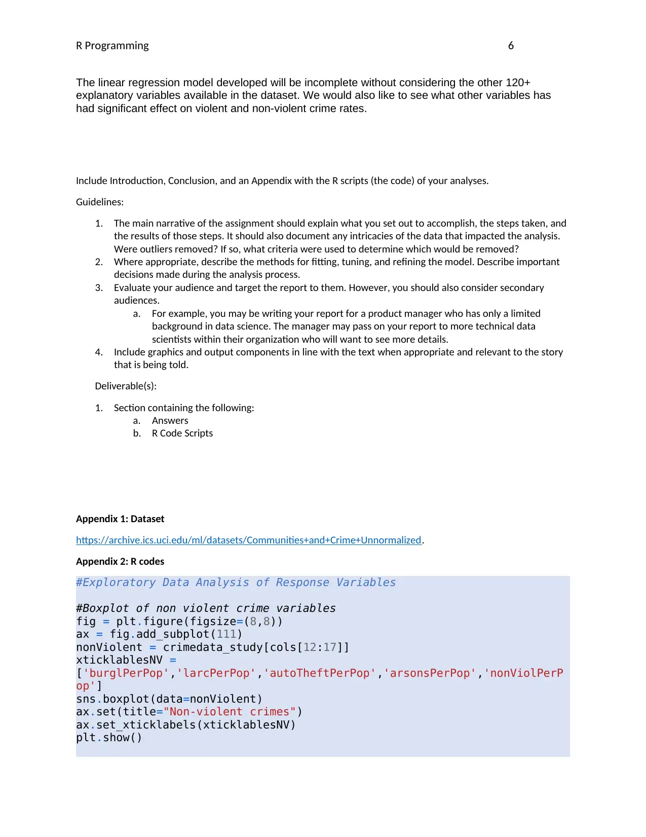
The linear regression model developed will be incomplete without considering the other 120+
explanatory variables available in the dataset. We would also like to see what other variables has
had significant effect on violent and non-violent crime rates.
Include Introduction, Conclusion, and an Appendix with the R scripts (the code) of your analyses.
Guidelines:
1. The main narrative of the assignment should explain what you set out to accomplish, the steps taken, and
the results of those steps. It should also document any intricacies of the data that impacted the analysis.
Were outliers removed? If so, what criteria were used to determine which would be removed?
2. Where appropriate, describe the methods for fitting, tuning, and refining the model. Describe important
decisions made during the analysis process.
3. Evaluate your audience and target the report to them. However, you should also consider secondary
audiences.
a. For example, you may be writing your report for a product manager who has only a limited
background in data science. The manager may pass on your report to more technical data
scientists within their organization who will want to see more details.
4. Include graphics and output components in line with the text when appropriate and relevant to the story
that is being told.
Deliverable(s):
1. Section containing the following:
a. Answers
b. R Code Scripts
Appendix 1: Dataset
https://archive.ics.uci.edu/ml/datasets/Communities+and+Crime+Unnormalized.
Appendix 2: R codes
#Exploratory Data Analysis of Response Variables
#Boxplot of non violent crime variables
fig = plt.figure(figsize=(8,8))
ax = fig.add_subplot(111)
nonViolent = crimedata_study[cols[12:17]]
xticklablesNV =
['burglPerPop','larcPerPop','autoTheftPerPop','arsonsPerPop','nonViolPerP
op']
sns.boxplot(data=nonViolent)
ax.set(title="Non-violent crimes")
ax.set_xticklabels(xticklablesNV)
plt.show()

R Programming 7
1 out of 7
Related Documents

Your All-in-One AI-Powered Toolkit for Academic Success.
+13062052269
info@desklib.com
Available 24*7 on WhatsApp / Email
![[object Object]](/_next/static/media/star-bottom.7253800d.svg)
Unlock your academic potential
© 2024 | Zucol Services PVT LTD | All rights reserved.