Statistical Analysis Using R: ANOVA, Kruskal-Wallis, Chi-Square

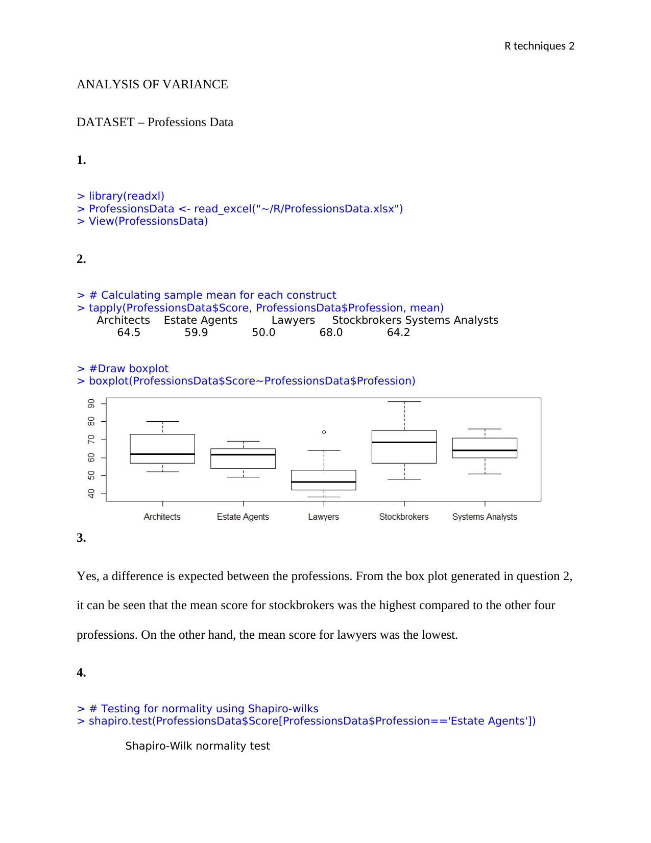
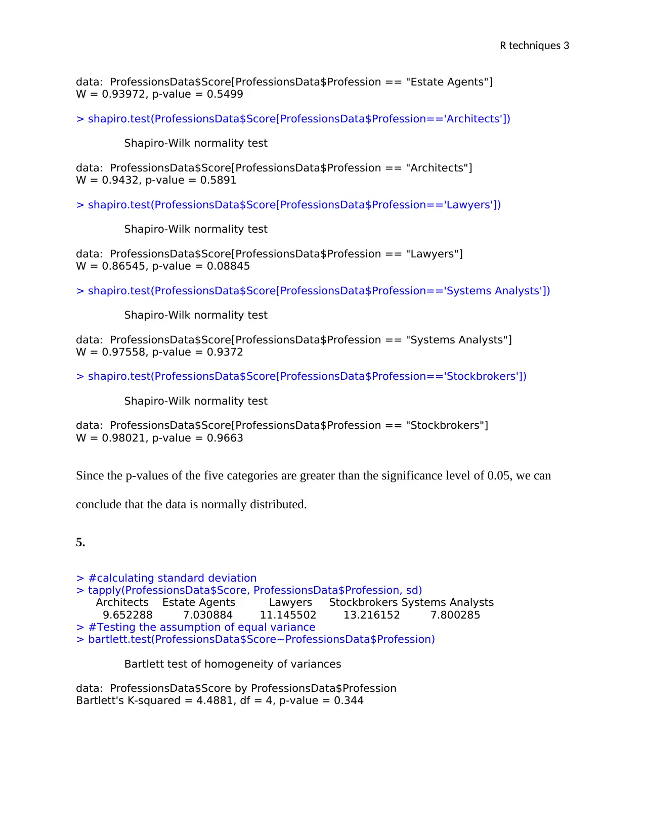
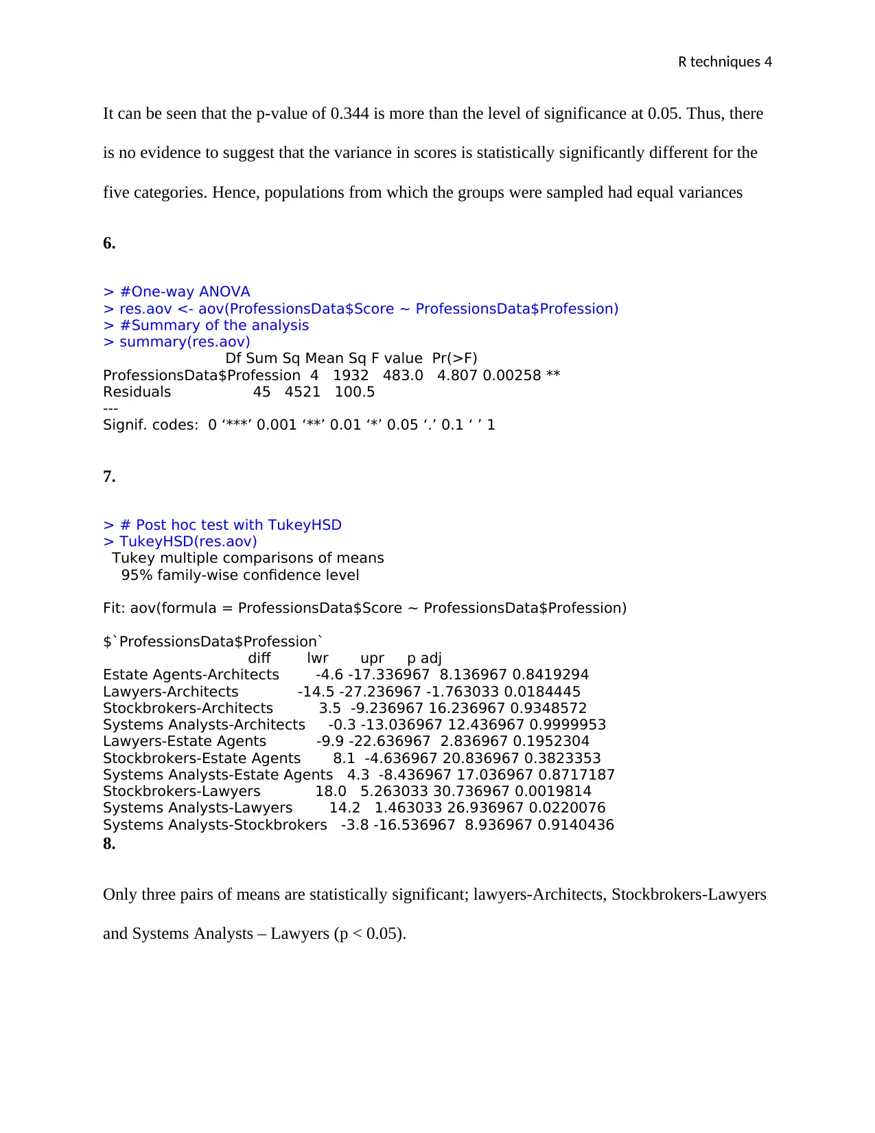
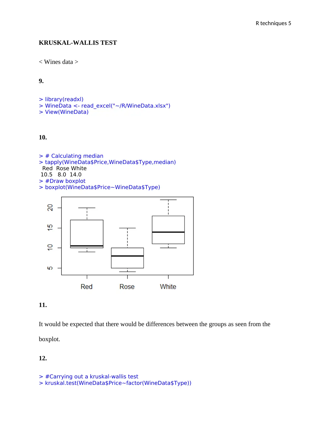
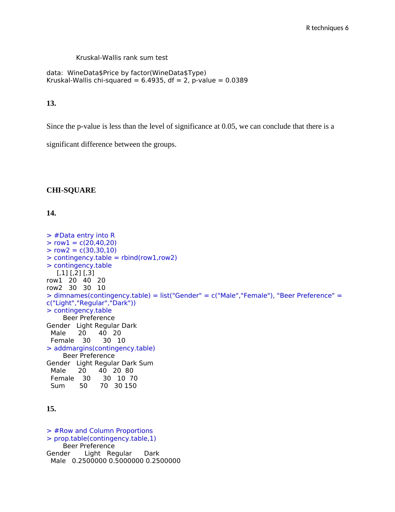
This assignment demonstrates the application of several statistical techniques using R. It includes an Analysis of Variance (ANOVA) to compare the mean scores of different professions, checking for normality and equal variance assumptions before conducting the ANOVA and post-hoc tests. Additionally, a Kruskal-Wallis test is performed to assess differences in wine prices across different types. Finally, a Chi-Square test is used to determine the dependence between gender and beer preference, including data entry, proportion calculations, graphical display, and interpretation of the test results. The assignment includes R code and interpretations of the output, providing a comprehensive guide to performing these statistical analyses in R.

Running Header: R techniques 1
R Techniques
Student’s Name:
Student’s ID:
Institution:

R techniques 2
ANALYSIS OF VARIANCE
DATASET – Professions Data
1.
> library(readxl)
> ProfessionsData <- read_excel("~/R/ProfessionsData.xlsx")
> View(ProfessionsData)
2.
> # Calculating sample mean for each construct
> tapply(ProfessionsData$Score, ProfessionsData$Profession, mean)
Architects Estate Agents Lawyers Stockbrokers Systems Analysts
64.5 59.9 50.0 68.0 64.2
> #Draw boxplot
> boxplot(ProfessionsData$Score~ProfessionsData$Profession)
3.
Yes, a difference is expected between the professions. From the box plot generated in question 2,
it can be seen that the mean score for stockbrokers was the highest compared to the other four
professions. On the other hand, the mean score for lawyers was the lowest.
4.
> # Testing for normality using Shapiro-wilks
> shapiro.test(ProfessionsData$Score[ProfessionsData$Profession=='Estate Agents'])
Shapiro-Wilk normality test

R techniques 3
data: ProfessionsData$Score[ProfessionsData$Profession == "Estate Agents"]
W = 0.93972, p-value = 0.5499
> shapiro.test(ProfessionsData$Score[ProfessionsData$Profession=='Architects'])
Shapiro-Wilk normality test
data: ProfessionsData$Score[ProfessionsData$Profession == "Architects"]
W = 0.9432, p-value = 0.5891
> shapiro.test(ProfessionsData$Score[ProfessionsData$Profession=='Lawyers'])
Shapiro-Wilk normality test
data: ProfessionsData$Score[ProfessionsData$Profession == "Lawyers"]
W = 0.86545, p-value = 0.08845
> shapiro.test(ProfessionsData$Score[ProfessionsData$Profession=='Systems Analysts'])
Shapiro-Wilk normality test
data: ProfessionsData$Score[ProfessionsData$Profession == "Systems Analysts"]
W = 0.97558, p-value = 0.9372
> shapiro.test(ProfessionsData$Score[ProfessionsData$Profession=='Stockbrokers'])
Shapiro-Wilk normality test
data: ProfessionsData$Score[ProfessionsData$Profession == "Stockbrokers"]
W = 0.98021, p-value = 0.9663
Since the p-values of the five categories are greater than the significance level of 0.05, we can
conclude that the data is normally distributed.
5.
> #calculating standard deviation
> tapply(ProfessionsData$Score, ProfessionsData$Profession, sd)
Architects Estate Agents Lawyers Stockbrokers Systems Analysts
9.652288 7.030884 11.145502 13.216152 7.800285
> #Testing the assumption of equal variance
> bartlett.test(ProfessionsData$Score~ProfessionsData$Profession)
Bartlett test of homogeneity of variances
data: ProfessionsData$Score by ProfessionsData$Profession
Bartlett's K-squared = 4.4881, df = 4, p-value = 0.344

R techniques 4
It can be seen that the p-value of 0.344 is more than the level of significance at 0.05. Thus, there
is no evidence to suggest that the variance in scores is statistically significantly different for the
five categories. Hence, populations from which the groups were sampled had equal variances
6.
> #One-way ANOVA
> res.aov <- aov(ProfessionsData$Score ~ ProfessionsData$Profession)
> #Summary of the analysis
> summary(res.aov)
Df Sum Sq Mean Sq F value Pr(>F)
ProfessionsData$Profession 4 1932 483.0 4.807 0.00258 **
Residuals 45 4521 100.5
---
Signif. codes: 0 ‘***’ 0.001 ‘**’ 0.01 ‘*’ 0.05 ‘.’ 0.1 ‘ ’ 1
7.
> # Post hoc test with TukeyHSD
> TukeyHSD(res.aov)
Tukey multiple comparisons of means
95% family-wise confidence level
Fit: aov(formula = ProfessionsData$Score ~ ProfessionsData$Profession)
$`ProfessionsData$Profession`
diff lwr upr p adj
Estate Agents-Architects -4.6 -17.336967 8.136967 0.8419294
Lawyers-Architects -14.5 -27.236967 -1.763033 0.0184445
Stockbrokers-Architects 3.5 -9.236967 16.236967 0.9348572
Systems Analysts-Architects -0.3 -13.036967 12.436967 0.9999953
Lawyers-Estate Agents -9.9 -22.636967 2.836967 0.1952304
Stockbrokers-Estate Agents 8.1 -4.636967 20.836967 0.3823353
Systems Analysts-Estate Agents 4.3 -8.436967 17.036967 0.8717187
Stockbrokers-Lawyers 18.0 5.263033 30.736967 0.0019814
Systems Analysts-Lawyers 14.2 1.463033 26.936967 0.0220076
Systems Analysts-Stockbrokers -3.8 -16.536967 8.936967 0.9140436
8.
Only three pairs of means are statistically significant; lawyers-Architects, Stockbrokers-Lawyers
and Systems Analysts – Lawyers (p < 0.05).

R techniques 5
KRUSKAL-WALLIS TEST
< Wines data >
9.
> library(readxl)
> WineData <- read_excel("~/R/WineData.xlsx")
> View(WineData)
10.
> # Calculating median
> tapply(WineData$Price,WineData$Type,median)
Red Rose White
10.5 8.0 14.0
> #Draw boxplot
> boxplot(WineData$Price~WineData$Type)
11.
It would be expected that there would be differences between the groups as seen from the
boxplot.
12.
> #Carrying out a kruskal-wallis test
> kruskal.test(WineData$Price~factor(WineData$Type))

R techniques 6
Kruskal-Wallis rank sum test
data: WineData$Price by factor(WineData$Type)
Kruskal-Wallis chi-squared = 6.4935, df = 2, p-value = 0.0389
13.
Since the p-value is less than the level of significance at 0.05, we can conclude that there is a
significant difference between the groups.
CHI-SQUARE
14.
> #Data entry into R
> row1 = c(20,40,20)
> row2 = c(30,30,10)
> contingency.table = rbind(row1,row2)
> contingency.table
[,1] [,2] [,3]
row1 20 40 20
row2 30 30 10
> dimnames(contingency.table) = list("Gender" = c("Male","Female"), "Beer Preference" =
c("Light","Regular","Dark"))
> contingency.table
Beer Preference
Gender Light Regular Dark
Male 20 40 20
Female 30 30 10
> addmargins(contingency.table)
Beer Preference
Gender Light Regular Dark Sum
Male 20 40 20 80
Female 30 30 10 70
Sum 50 70 30 150
15.
> #Row and Column Proportions
> prop.table(contingency.table,1)
Beer Preference
Gender Light Regular Dark
Male 0.2500000 0.5000000 0.2500000

R techniques 7
Female 0.4285714 0.4285714 0.1428571
> prop.table(contingency.table,2)
Beer Preference
Gender Light Regular Dark
Male 0.4 0.5714286 0.6666667
Female 0.6 0.4285714 0.3333333
> #Overall Proportions
> prop.table(contingency.table)
Beer Preference
Gender Light Regular Dark
Male 0.1333333 0.2666667 0.13333333
Female 0.2000000 0.2000000 0.06666667
16.
> #Graphical display of data
> barplot(contingency.table, beside=T, legend=T,ylab="Observed frequencies",
main="Frequency of Beer Preference by Gender")
From the plotted graph, it could be seen that there is no discernable association between the beer
preference and gender.
17.
> #Chi-square test
> chisq.test(contingency.table)
Pearson's Chi-squared test
data: contingency.table
X-squared = 6.1224, df = 2, p-value = 0.04683

R techniques 8
18.
The obtained chi-squared value is 6.1224. Since the p-value is less than the level of significance
at 0.05, we choose to reject the null hypothesis hence concluding that the two variable are
dependent.