Race Vehicle Testing
VerifiedAdded on 2023/04/21
|18
|4122
|260
AI Summary
This document discusses race vehicle testing and analysis, including sensors and instrumentation, different sensors and their features, steering wheel angle calibration, yaw angle calculation, Kalman filter design, path curvature calculation, and comparison of maximum speed and actual speed. The document provides explanations, MATLAB code, and plots for each topic.
Contribute Materials
Your contribution can guide someone’s learning journey. Share your
documents today.
Race vehicle testing
Secure Best Marks with AI Grader
Need help grading? Try our AI Grader for instant feedback on your assignments.
Table of Contents
Introduction.........................................................................................................................................3
Description...........................................................................................................................................3
Question 1:...........................................................................................................................................3
Sensors and instrumentation background and implementation..................................................3
Question 2:...........................................................................................................................................4
Different Sensors and its features...................................................................................................4
Question 3:...........................................................................................................................................5
Steering wheel angle........................................................................................................................5
Question 4:...........................................................................................................................................6
Yaw angle.........................................................................................................................................6
Question 5:...........................................................................................................................................7
Kalman filter design........................................................................................................................7
Question 6:...........................................................................................................................................8
Path Curvature................................................................................................................................8
Question 7:...........................................................................................................................................9
Comparison of maximum speed and actual speed........................................................................9
Question 8:.........................................................................................................................................10
Driver input and vehicle response................................................................................................10
Conclusion:........................................................................................................................................12
Appendix............................................................................................................................................13
Outputs...........................................................................................................................................13
Introduction
A sensor is a device which detects and respond to the information received. It
measures on various parameters like property, colour, frequency etc. The sensor
has the capability of converting an input signal (stimulus) into a measured
signal. The input signal or stimulus is mechanical, thermal, electromagnetic,
acoustic or chemical in nature. Whereas the measured signal is electrical in
nature. The essential component of engineering devices are sensors. It is based
on a wide range of physical principles.
Description
The description of the project is to analyse different parameters for a race car.
The testing assessment is mainly based on steering angle, yaw angle, path
curvature, speed of a car for different values of acceleration. The filter is also
used in analysis when there is any disturbance occurs during the drive.
Question 1:
Sensors and instrumentation background and implementation
Answer:
The sensors in the instrument or in the device can be communicated in a real-
time application through graphical instrument panels. MATLAB makes a
feature of its professional toolboxes which function is powerful. The Real time
system monitoring is a challenging task for every analysis. It is therefore a
multidisciplinary application. The data is downloaded from FTP server. And
then it is decoded to specified format. Then the report is fed into different
Database and presentation purposes. These data are used in real time
applications. The application of sensor in Matlab can be implemented either
through Matlab / Simlink or through Matlab toolbox i,e GUI (Graphical User
Interface). MATLAB Tool were used to download data from FTP server and
decode ASCII character in to hex and decimal form for further analysis. The
sensor implementation is explained through nodes which can be detected by
sensor only in a definite path.
Question 2:
Different Sensors and its features
Explain and report on the various commercially available unit of different
sensors and DAQ devices, principles of operation, features, properties, and
problems.
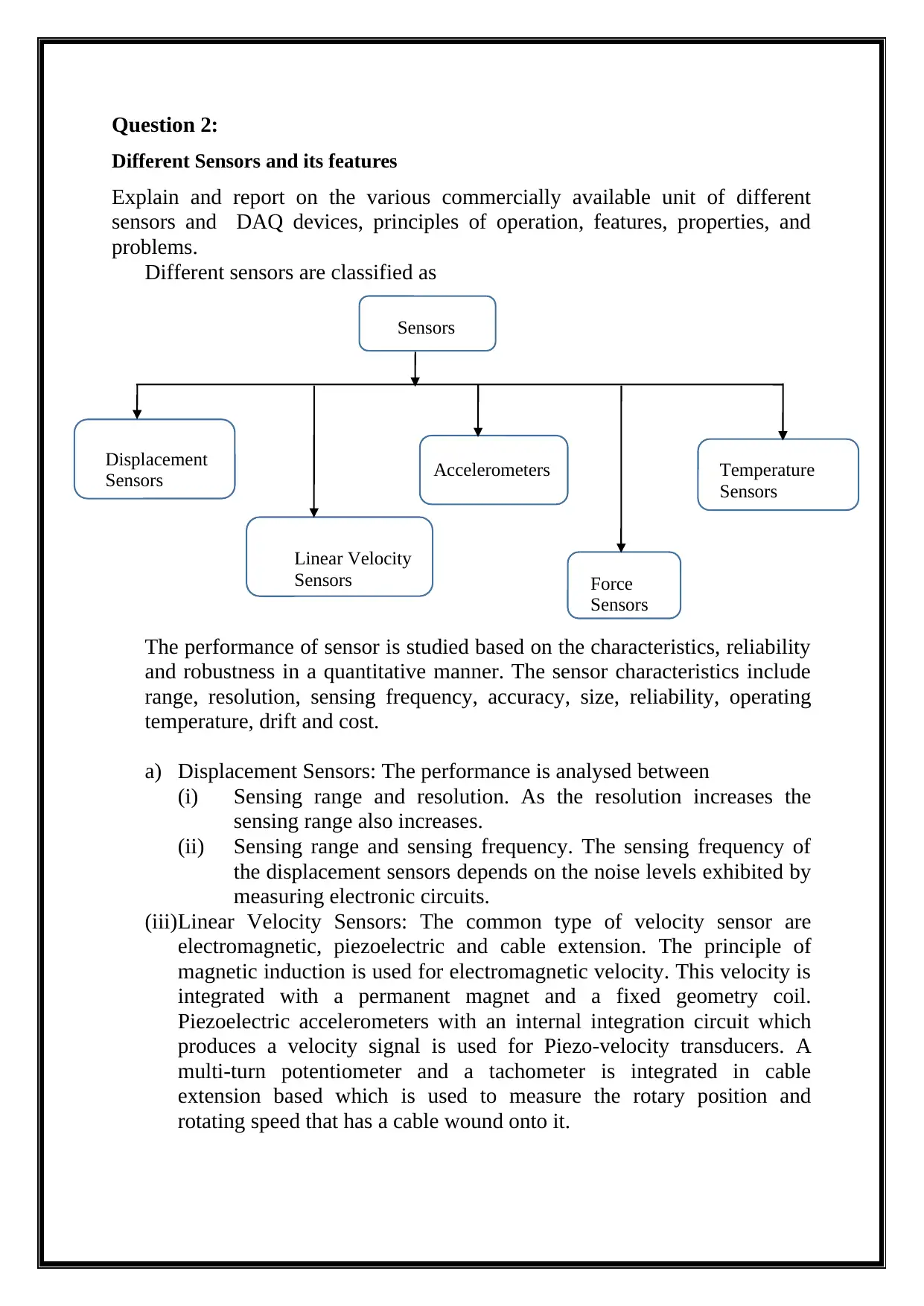
Different sensors are classified as
The performance of sensor is studied based on the characteristics, reliability
and robustness in a quantitative manner. The sensor characteristics include
range, resolution, sensing frequency, accuracy, size, reliability, operating
temperature, drift and cost.
a) Displacement Sensors: The performance is analysed between
(i) Sensing range and resolution. As the resolution increases the
sensing range also increases.
(ii) Sensing range and sensing frequency. The sensing frequency of
the displacement sensors depends on the noise levels exhibited by
measuring electronic circuits.
(iii)Linear Velocity Sensors: The common type of velocity sensor are
electromagnetic, piezoelectric and cable extension. The principle of
magnetic induction is used for electromagnetic velocity. This velocity is
integrated with a permanent magnet and a fixed geometry coil.
Piezoelectric accelerometers with an internal integration circuit which
produces a velocity signal is used for Piezo-velocity transducers. A
multi-turn potentiometer and a tachometer is integrated in cable
extension based which is used to measure the rotary position and
rotating speed that has a cable wound onto it.
Sensors
Displacement
Sensors
Linear Velocity
Sensors
Accelerometers
Force
Sensors
Temperature
Sensors
Different Sensors and its features
Explain and report on the various commercially available unit of different
sensors and DAQ devices, principles of operation, features, properties, and
problems.
Different sensors are classified as
The performance of sensor is studied based on the characteristics, reliability
and robustness in a quantitative manner. The sensor characteristics include
range, resolution, sensing frequency, accuracy, size, reliability, operating
temperature, drift and cost.
a) Displacement Sensors: The performance is analysed between
(i) Sensing range and resolution. As the resolution increases the
sensing range also increases.
(ii) Sensing range and sensing frequency. The sensing frequency of
the displacement sensors depends on the noise levels exhibited by
measuring electronic circuits.
(iii)Linear Velocity Sensors: The common type of velocity sensor are
electromagnetic, piezoelectric and cable extension. The principle of
magnetic induction is used for electromagnetic velocity. This velocity is
integrated with a permanent magnet and a fixed geometry coil.
Piezoelectric accelerometers with an internal integration circuit which
produces a velocity signal is used for Piezo-velocity transducers. A
multi-turn potentiometer and a tachometer is integrated in cable
extension based which is used to measure the rotary position and
rotating speed that has a cable wound onto it.
Sensors
Displacement
Sensors
Linear Velocity
Sensors
Accelerometers
Force
Sensors
Temperature
Sensors
Secure Best Marks with AI Grader
Need help grading? Try our AI Grader for instant feedback on your assignments.
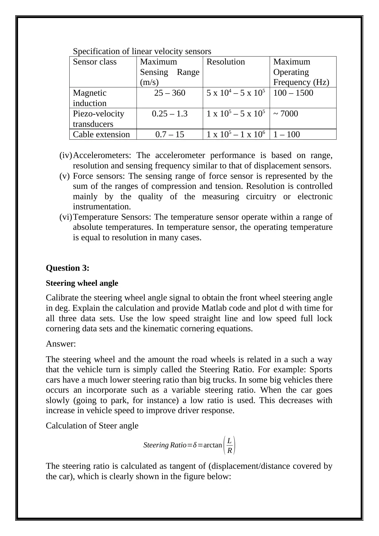
Specification of linear velocity sensors
Sensor class Maximum
Sensing Range
(m/s)
Resolution Maximum
Operating
Frequency (Hz)
Magnetic
induction
25 – 360 5 x 10⁴ – 5 x 10⁵ 100 – 1500
Piezo-velocity
transducers
0.25 – 1.3 1 x 10⁵ – 5 x 10⁵ ~ 7000
Cable extension 0.7 – 15 1 x 10⁵ – 1 x 10⁶ 1 – 100
(iv)Accelerometers: The accelerometer performance is based on range,
resolution and sensing frequency similar to that of displacement sensors.
(v) Force sensors: The sensing range of force sensor is represented by the
sum of the ranges of compression and tension. Resolution is controlled
mainly by the quality of the measuring circuitry or electronic
instrumentation.
(vi)Temperature Sensors: The temperature sensor operate within a range of
absolute temperatures. In temperature sensor, the operating temperature
is equal to resolution in many cases.
Question 3:
Steering wheel angle
Calibrate the steering wheel angle signal to obtain the front wheel steering angle
in deg. Explain the calculation and provide Matlab code and plot d with time for
all three data sets. Use the low speed straight line and low speed full lock
cornering data sets and the kinematic cornering equations.
Answer:
The steering wheel and the amount the road wheels is related in a such a way
that the vehicle turn is simply called the Steering Ratio. For example: Sports
cars have a much lower steering ratio than big trucks. In some big vehicles there
occurs an incorporate such as a variable steering ratio. When the car goes
slowly (going to park, for instance) a low ratio is used. This decreases with
increase in vehicle speed to improve driver response.
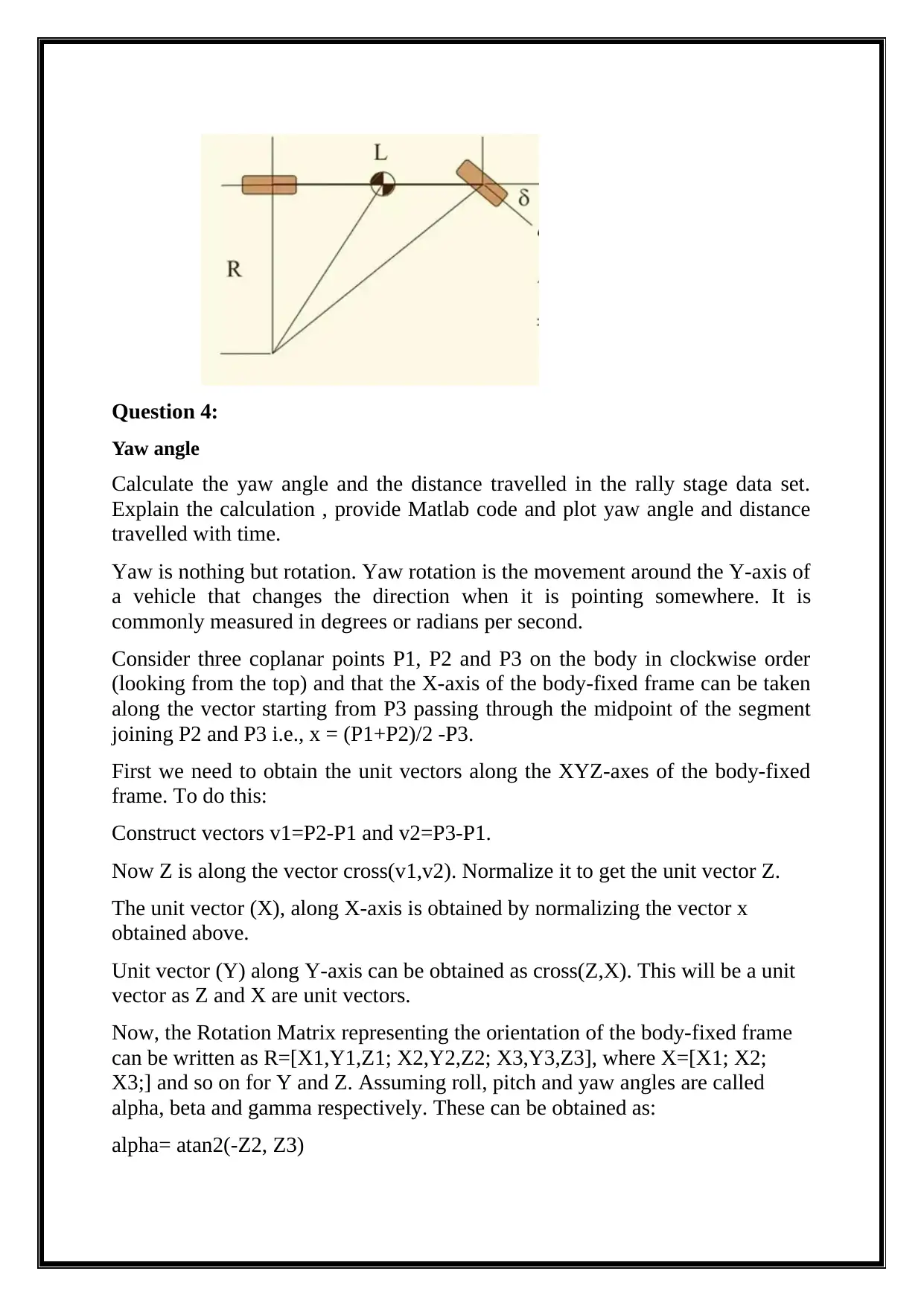
Calculation of Steer angle
Steering Ratio=δ =arctan ( L
R )
The steering ratio is calculated as tangent of (displacement/distance covered by
the car), which is clearly shown in the figure below:
Sensor class Maximum
Sensing Range
(m/s)
Resolution Maximum
Operating
Frequency (Hz)
Magnetic
induction
25 – 360 5 x 10⁴ – 5 x 10⁵ 100 – 1500
Piezo-velocity
transducers
0.25 – 1.3 1 x 10⁵ – 5 x 10⁵ ~ 7000
Cable extension 0.7 – 15 1 x 10⁵ – 1 x 10⁶ 1 – 100
(iv)Accelerometers: The accelerometer performance is based on range,
resolution and sensing frequency similar to that of displacement sensors.
(v) Force sensors: The sensing range of force sensor is represented by the
sum of the ranges of compression and tension. Resolution is controlled
mainly by the quality of the measuring circuitry or electronic
instrumentation.
(vi)Temperature Sensors: The temperature sensor operate within a range of
absolute temperatures. In temperature sensor, the operating temperature
is equal to resolution in many cases.
Question 3:
Steering wheel angle
Calibrate the steering wheel angle signal to obtain the front wheel steering angle
in deg. Explain the calculation and provide Matlab code and plot d with time for
all three data sets. Use the low speed straight line and low speed full lock
cornering data sets and the kinematic cornering equations.
Answer:
The steering wheel and the amount the road wheels is related in a such a way
that the vehicle turn is simply called the Steering Ratio. For example: Sports
cars have a much lower steering ratio than big trucks. In some big vehicles there
occurs an incorporate such as a variable steering ratio. When the car goes
slowly (going to park, for instance) a low ratio is used. This decreases with
increase in vehicle speed to improve driver response.
Calculation of Steer angle
Steering Ratio=δ =arctan ( L
R )
The steering ratio is calculated as tangent of (displacement/distance covered by
the car), which is clearly shown in the figure below:
Question 4:
Yaw angle
Calculate the yaw angle and the distance travelled in the rally stage data set.
Explain the calculation , provide Matlab code and plot yaw angle and distance
travelled with time.
Yaw is nothing but rotation. Yaw rotation is the movement around the Y-axis of
a vehicle that changes the direction when it is pointing somewhere. It is
commonly measured in degrees or radians per second.
Consider three coplanar points P1, P2 and P3 on the body in clockwise order
(looking from the top) and that the X-axis of the body-fixed frame can be taken
along the vector starting from P3 passing through the midpoint of the segment
joining P2 and P3 i.e., x = (P1+P2)/2 -P3.
First we need to obtain the unit vectors along the XYZ-axes of the body-fixed
frame. To do this:
Construct vectors v1=P2-P1 and v2=P3-P1.
Now Z is along the vector cross(v1,v2). Normalize it to get the unit vector Z.
The unit vector (X), along X-axis is obtained by normalizing the vector x
obtained above.
Unit vector (Y) along Y-axis can be obtained as cross(Z,X). This will be a unit
vector as Z and X are unit vectors.
Now, the Rotation Matrix representing the orientation of the body-fixed frame
can be written as R=[X1,Y1,Z1; X2,Y2,Z2; X3,Y3,Z3], where X=[X1; X2;
X3;] and so on for Y and Z. Assuming roll, pitch and yaw angles are called
alpha, beta and gamma respectively. These can be obtained as:
alpha= atan2(-Z2, Z3)
beta= asin(Z1)
gamma = atan2(-Y1,X1)
Question 5:
Kalman filter design
Design a software filter for the longitudinal/lateral acceleration signals in the
rally stage data set. Explain the calculation, provide Matlab code and compare
filtered and unfiltered signals in the same plot.
Kalman filter is a suitable for the system which is corrupted with the Gaussian
noise. This filter is a recursive state space model based of algorithm. The
algorithm was basically developed for single dimensional and real valued
signals which are associated with the linear systems. The Kalman filter
estimates the discrete – time controlled process which is governed by the linear
difference equation
xk= A xk−1 +B uk−1 +wk−1
with a measurement z which is given as
zk=Hxk+ vk
The random variables wk and vk represent the process noise and measurement
noise respectively.
The true motion of the vehicle can be estimated using a kinematics approach.
The vehicle is considered a rigid body and the wheels of the vehicle are
considered for the estimation.⃗
υf =
[ υx
υ y + Lf r ]⃗
υr= [ υ x
υy−Lr r ]
The value of υx and υ y are calculated as:
[υx
υy ]=
[ Rω ωf cos δf + Rω ωr
2
Rω ωf sin δf −Lf r + Lr r
2 ]
Paraphrase This Document
Need a fresh take? Get an instant paraphrase of this document with our AI Paraphraser
Question 6:
Path Curvature
Calculate the path curvature k in the rally stage data and plot k with distance
travelled s. Explain the calculation and provide Matlab code. Use vehicle speed,
sideslip, and body acceleration signals.
Answer:
A self driving car starts with the perception system, which is use to estimate the
state of the surrounding environment, including landmarks and vehicles and
pedestrians. The localization block compares a map to figure out to locate the
distance of the vehicle. After calculating the vehicle’s location, the path is
planned to find a trajectory to the destination. The steering and throttle/brake at
every time step is used to control and guide the vehicle on this trajectory.
Implementation of predictive control is used to drive the car around. The
simulator provides position and velocity of the car at each time step back to the
user. In turn the user provides the steering and acceleration to the simulator to
apply to the car. State of the vehicle at any point is described by 4 vectors — x
position, y position, velocity (v) and the orientation (psi). Actuators or control
inputs are the steering angle (delta) and the throttle value (a). Braking can be
expressed as negative throttle. Throttle have values between -1 an +1. Steering
angle is set to the angle between -30 deg to +30 deg.
The Kinematic motion model is used to predict new state from previous state
after steering and throttle are applied.
x_[t+1] = x[t] + v[t] * cos(psi[t]) * dt
y_[t+1] = y[t] + v[t] * sin(psi[t]) * dt
psi_[t+1] = psi[t] + v[t] / Lf * delta[t] * dt
v_[t+1] = v[t] + a[t] * dt
Where Lf is the distance between the front of the vehicle and its centre of
gravity. The larger the vehicle, the slower the turn rate. The ideal steering angle
and throttle can be estimated as the error of our new state from our ideal state.
Actual trajectory to be followed and to maintain the velocity and orientation, a
solver is used to minimize this error. This helps to select the steering and
throttle that minimizes the error with the desired trajectory. Errors are based on
the following:
Distance from the reference: The equation below depicts this error.
Orientation error¿ cosθ +εi (t )
The error can be summed up due to difference with respect to x and y .
Difference from desired orientation is defined as the orientation error (epsi) and
difference from reference velocity.
Error in proportion to change in actuators: This is the cost function that captures
the difference between the next actuator state and the current one. This ensures
smooth changes in actuator values. The above states can be multiplied by
weights and these weights increase the importance of the term in the overall
cost equation. Two other fairly important parameters are given as: number of
time steps in to the future (N) used to predict steering and throttle. And time
step length (dt).
dt— It is the time gap between different time steps. It isa very important
parameter for the overall performance in the simulator. If dt is too low, the car
leads to oscillate to and fro around the center of the track. This happens
probably because the actuator input is received very quickly and the vehicle is
constantly responding. Also if dt is smaller than the latency (0.1 s) then the new
actuator signal is received before the previous one was executed. This leads to
jerks in the motion of the car. On the other hand if dt is too large, the car covers
too much distance before the actuator is received and this leads to smooth
performance along the straight portions of the track and therefore this leads to
car going off the road on the curves.
N — Is the number of time steps to the model that predicts ahead. The model
predicts further ahead with increase in N. The more inaccurate the predictions
with the prediction of the model. A lot of computations has to be done for larger
values of N which can lead to inaccurate results from the solver or solver unable
to provide the solution in real time.
Question 7:
Comparison of maximum speed and actual speed
Isolate a full lap through the rally stage and assign a value of local maximum
magnitude of curvature at each corner of the circuit. Using the maximum
observed cornering acceleration, calculate the theoretical maximum allowable
speed individually at each corner and compare it with the actual speed achieved
by the driver.
Answer:
A car entering curve from a straight line, from curve to another curve with
different radius and leaving a curve to enter a straight line are types of sudden
changes and this causes discomfort to driver. Therefore, a transition curve from
one form to another is needed. A transition curve is constructed in the route
design for highway and railways. It is important to have joining curve between
two different arc lengths. In curve and surface design, it is desirable to have
planar transition curve, where transition curve between two circles can combine
to form C-shape curve and S-shape curve. The planar transition consist of circle
to straight lines or vice-versa and circle to circle with different radius.
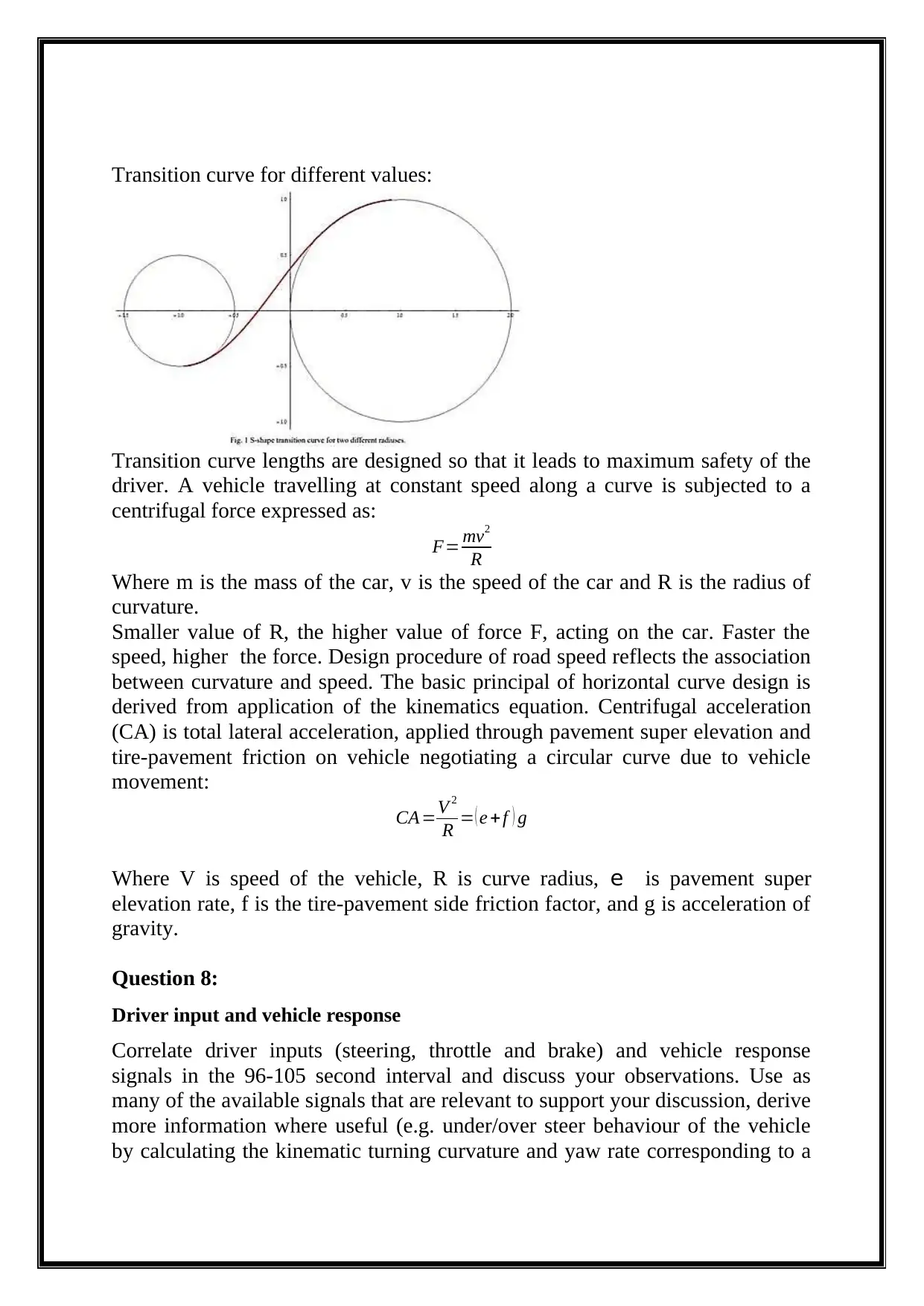
Transition curve for different values:
Transition curve lengths are designed so that it leads to maximum safety of the
driver. A vehicle travelling at constant speed along a curve is subjected to a
centrifugal force expressed as:
F= mv2
R
Where m is the mass of the car, v is the speed of the car and R is the radius of
curvature.
Smaller value of R, the higher value of force F, acting on the car. Faster the
speed, higher the force. Design procedure of road speed reflects the association
between curvature and speed. The basic principal of horizontal curve design is
derived from application of the kinematics equation. Centrifugal acceleration
(CA) is total lateral acceleration, applied through pavement super elevation and
tire-pavement friction on vehicle negotiating a circular curve due to vehicle
movement:
CA =V 2
R = ( e + f ) g
Where V is speed of the vehicle, R is curve radius, e is pavement super
elevation rate, f is the tire-pavement side friction factor, and g is acceleration of
gravity.
Question 8:
Driver input and vehicle response
Correlate driver inputs (steering, throttle and brake) and vehicle response
signals in the 96-105 second interval and discuss your observations. Use as
many of the available signals that are relevant to support your discussion, derive
more information where useful (e.g. under/over steer behaviour of the vehicle
by calculating the kinematic turning curvature and yaw rate corresponding to a
Secure Best Marks with AI Grader
Need help grading? Try our AI Grader for instant feedback on your assignments.
neutral steer car), interpret the vehicle response to the given driver inputs and
provide the necessary plots. Use distance plots rather than time plots.
Answer:
Self driving car follows a path just like a 4 wheeled robot The path can be
calculated globally, say from one point to another point like a taxi and/or
locally, going forward in a highway without departing the lane. In this process,
the car should adapt its speed and do not hit objects and plan its path to avoid
obstacles.
Let us consider the simplest case possible. A car in a highway without any other
vehicles in and around. And want it to go forward keeping itself in the centre of
the lane. A human could solve the problem and maintain its speed of a car in the
centre of a lane. It has to be checked regularly, the distance from left and right
lanes. If it is close to the left lane, steer the vehicle to the right and vice-versa.
Normal human eyes and spatial intelligence can be used to estimate the lane
distance. Similarly speed also estimated in the same form. If the speed of the car
is too slow, to release the gas the brake has to be pressed. The intuition involves
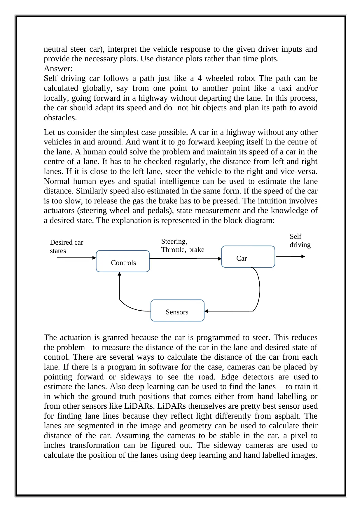
actuators (steering wheel and pedals), state measurement and the knowledge of
a desired state. The explanation is represented in the block diagram:
The actuation is granted because the car is programmed to steer. This reduces
the problem to measure the distance of the car in the lane and desired state of
control. There are several ways to calculate the distance of the car from each
lane. If there is a program in software for the case, cameras can be placed by
pointing forward or sideways to see the road. Edge detectors are used to
estimate the lanes. Also deep learning can be used to find the lanes — to train it
in which the ground truth positions that comes either from hand labelling or
from other sensors like LiDARs. LiDARs themselves are pretty best sensor used
for finding lane lines because they reflect light differently from asphalt. The
lanes are segmented in the image and geometry can be used to calculate their
distance of the car. Assuming the cameras to be stable in the car, a pixel to
inches transformation can be figured out. The sideway cameras are used to
calculate the position of the lanes using deep learning and hand labelled images.
Controls Car
Desired car
states
Steering,
Throttle, brake
Self
driving
Sensors
provide the necessary plots. Use distance plots rather than time plots.
Answer:
Self driving car follows a path just like a 4 wheeled robot The path can be
calculated globally, say from one point to another point like a taxi and/or
locally, going forward in a highway without departing the lane. In this process,
the car should adapt its speed and do not hit objects and plan its path to avoid
obstacles.
Let us consider the simplest case possible. A car in a highway without any other
vehicles in and around. And want it to go forward keeping itself in the centre of
the lane. A human could solve the problem and maintain its speed of a car in the
centre of a lane. It has to be checked regularly, the distance from left and right
lanes. If it is close to the left lane, steer the vehicle to the right and vice-versa.
Normal human eyes and spatial intelligence can be used to estimate the lane
distance. Similarly speed also estimated in the same form. If the speed of the car
is too slow, to release the gas the brake has to be pressed. The intuition involves
actuators (steering wheel and pedals), state measurement and the knowledge of
a desired state. The explanation is represented in the block diagram:
The actuation is granted because the car is programmed to steer. This reduces
the problem to measure the distance of the car in the lane and desired state of
control. There are several ways to calculate the distance of the car from each
lane. If there is a program in software for the case, cameras can be placed by
pointing forward or sideways to see the road. Edge detectors are used to
estimate the lanes. Also deep learning can be used to find the lanes — to train it
in which the ground truth positions that comes either from hand labelling or
from other sensors like LiDARs. LiDARs themselves are pretty best sensor used
for finding lane lines because they reflect light differently from asphalt. The
lanes are segmented in the image and geometry can be used to calculate their
distance of the car. Assuming the cameras to be stable in the car, a pixel to
inches transformation can be figured out. The sideway cameras are used to
calculate the position of the lanes using deep learning and hand labelled images.
Controls Car
Desired car
states
Steering,
Throttle, brake
Self
driving
Sensors
Speed measurement is easy to estimate which is already provided by the car
internals. After determining the position and speed of the car in the road, the
desired position can be controlled with respect to the speed. Another solution to
the problem can be found by simply assuming dividing the problem in to two
parts: Longitudinal (throttle and brake) and Lateral (torque on the steering
wheels) controls. The break down does not work always.
Conclusion:
The testing assessment is made for a race car. The steering angle, the yaw angle
for different values of distance are measured and plotted in the graph. The filter
called Kalman filter is deigned in order to reduce the disturbance or noise when
the vehicle runs with actuators or sensors. Different types of sensors and its
characteristics are studied. The response for various driver inputs is analysed.
Appendix
Outputs
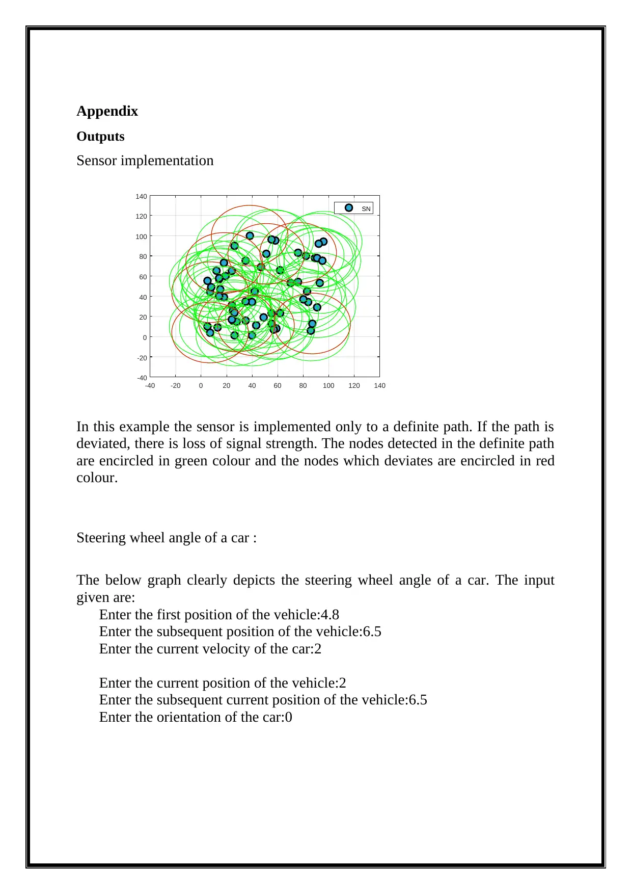
Sensor implementation
In this example the sensor is implemented only to a definite path. If the path is
deviated, there is loss of signal strength. The nodes detected in the definite path
are encircled in green colour and the nodes which deviates are encircled in red
colour.
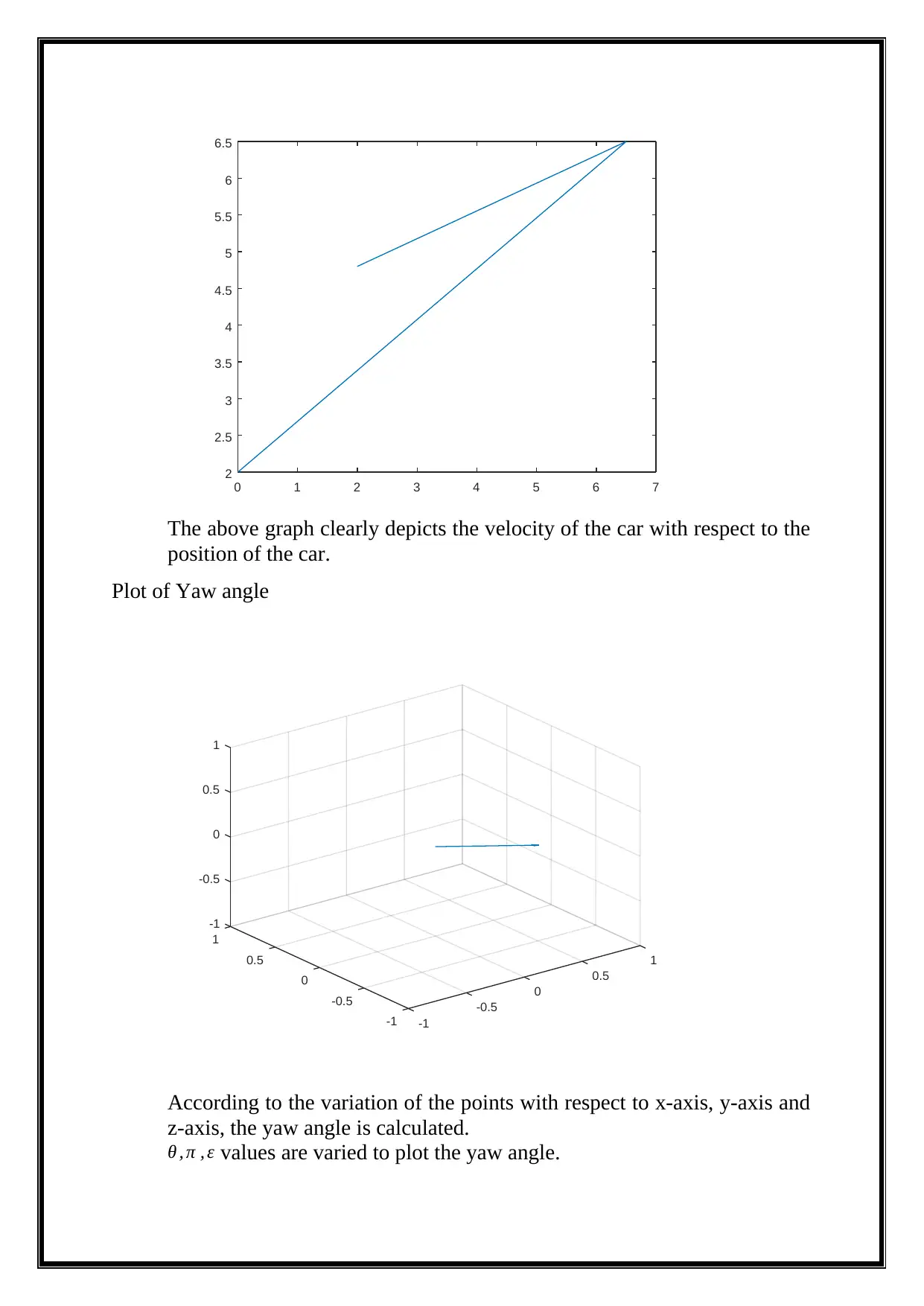
Steering wheel angle of a car :
The below graph clearly depicts the steering wheel angle of a car. The input
given are:
Enter the first position of the vehicle:4.8
Enter the subsequent position of the vehicle:6.5
Enter the current velocity of the car:2
Enter the current position of the vehicle:2
Enter the subsequent current position of the vehicle:6.5
Enter the orientation of the car:0
-40 -20 0 20 40 60 80 100 120 140
-40
-20
0
20
40
60
80
100
120
140
SN
Outputs
Sensor implementation
In this example the sensor is implemented only to a definite path. If the path is
deviated, there is loss of signal strength. The nodes detected in the definite path
are encircled in green colour and the nodes which deviates are encircled in red
colour.
Steering wheel angle of a car :
The below graph clearly depicts the steering wheel angle of a car. The input
given are:
Enter the first position of the vehicle:4.8
Enter the subsequent position of the vehicle:6.5
Enter the current velocity of the car:2
Enter the current position of the vehicle:2
Enter the subsequent current position of the vehicle:6.5
Enter the orientation of the car:0
-40 -20 0 20 40 60 80 100 120 140
-40
-20
0
20
40
60
80
100
120
140
SN
Paraphrase This Document
Need a fresh take? Get an instant paraphrase of this document with our AI Paraphraser
0 1 2 3 4 5 6 7
2
2.5
3
3.5
4
4.5
5
5.5
6
6.5
The above graph clearly depicts the velocity of the car with respect to the
position of the car.
Plot of Yaw angle
According to the variation of the points with respect to x-axis, y-axis and
z-axis, the yaw angle is calculated.
θ , π , ε values are varied to plot the yaw angle.
1
0.5
0
-0.5
-1-1
-0.5
0
0.5
-1
-0.5
0
0.5
1
1
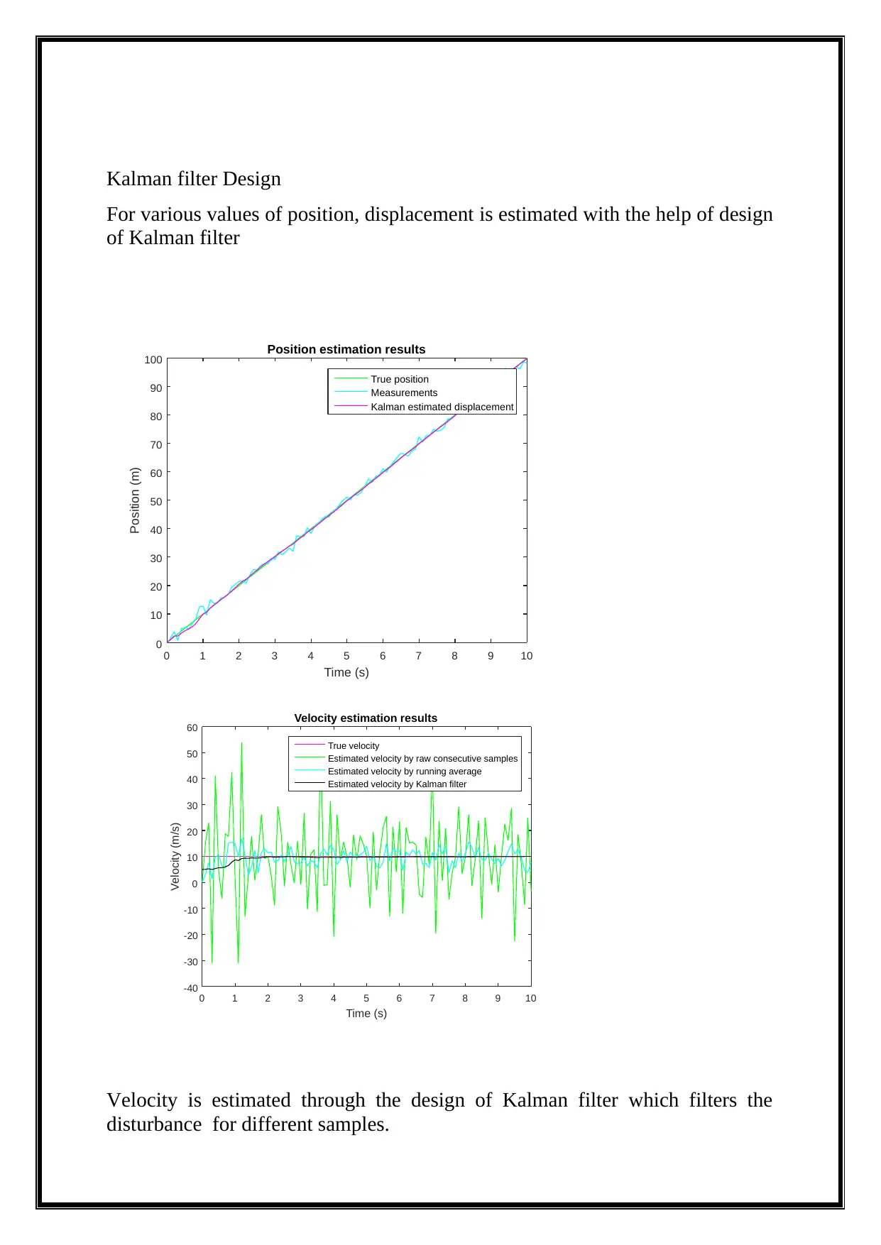
Kalman filter Design
For various values of position, displacement is estimated with the help of design
of Kalman filter
Time (s)
0 1 2 3 4 5 6 7 8 9 10
Position (m)
0
10
20
30
40
50
60
70
80
90
100 Position estimation results
True position
Measurements
Kalman estimated displacement
Velocity is estimated through the design of Kalman filter which filters the
disturbance for different samples.
Time (s)
0 1 2 3 4 5 6 7 8 9 10
Velocity (m/s)
-40
-30
-20
-10
0
10
20
30
40
50
60 Velocity estimation results
True velocity
Estimated velocity by raw consecutive samples
Estimated velocity by running average
Estimated velocity by Kalman filter
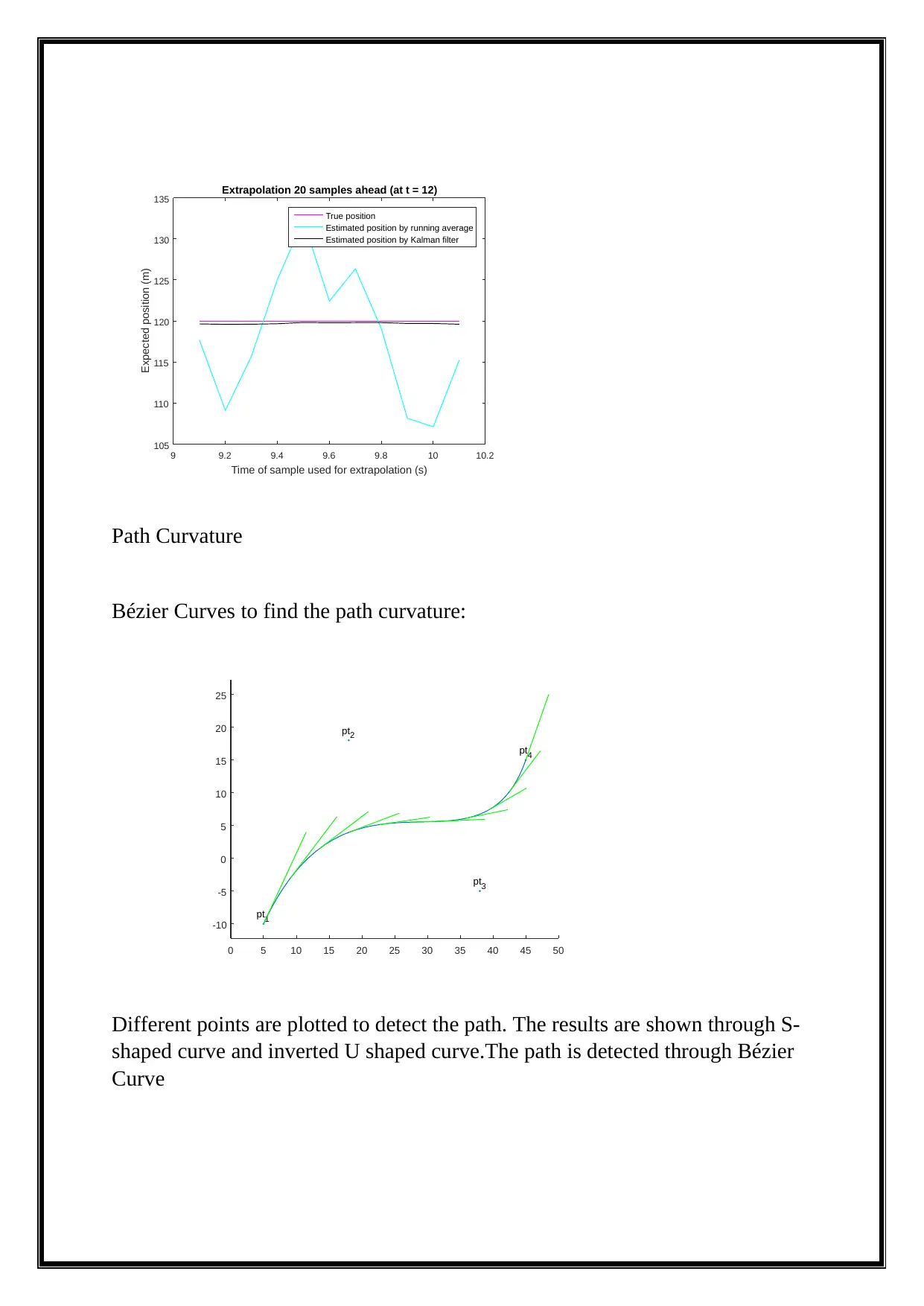
Path Curvature
Bézier Curves to find the path curvature:
Different points are plotted to detect the path. The results are shown through S-
shaped curve and inverted U shaped curve.The path is detected through Bézier
Curve
Time of sample used for extrapolation (s)
9 9.2 9.4 9.6 9.8 10 10.2
Expected position (m)
105
110
115
120
125
130
135 Extrapolation 20 samples ahead (at t = 12)
True position
Estimated position by running average
Estimated position by Kalman filter
0 5 10 15 20 25 30 35 40 45 50
-10
-5
0
5
10
15
20
25
pt1
pt2
pt3
pt4
Secure Best Marks with AI Grader
Need help grading? Try our AI Grader for instant feedback on your assignments.
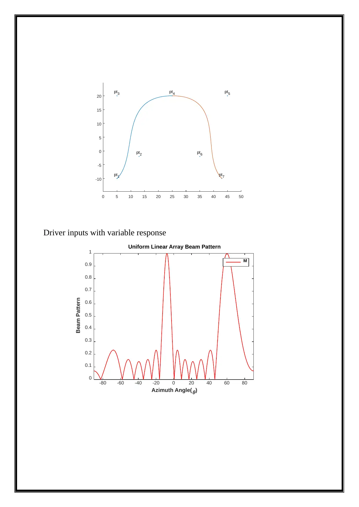
Driver inputs with variable response
Azimuth Angle( )
-80 -60 -40 -20 0 20 40 60 80
Beam Pattern
0
0.1
0.2
0.3
0.4
0.5
0.6
0.7
0.8
0.9
1
Uniform Linear Array Beam Pattern
M
0 5 10 15 20 25 30 35 40 45 50
-10
-5
0
5
10
15
20
pt1
pt2
pt3 pt4 pt5
pt6
pt7
Azimuth Angle( )
-80 -60 -40 -20 0 20 40 60 80
Beam Pattern
0
0.1
0.2
0.3
0.4
0.5
0.6
0.7
0.8
0.9
1
Uniform Linear Array Beam Pattern
M
0 5 10 15 20 25 30 35 40 45 50
-10
-5
0
5
10
15
20
pt1
pt2
pt3 pt4 pt5
pt6
pt7
Spatial Frequency(fs)
-1 -0.8 -0.6 -0.4 -0.2 0 0.2 0.4 0.6 0.8 1
Beam Pattern
0
0.1
0.2
0.3
0.4
0.5
0.6
0.7
0.8
0.9
1
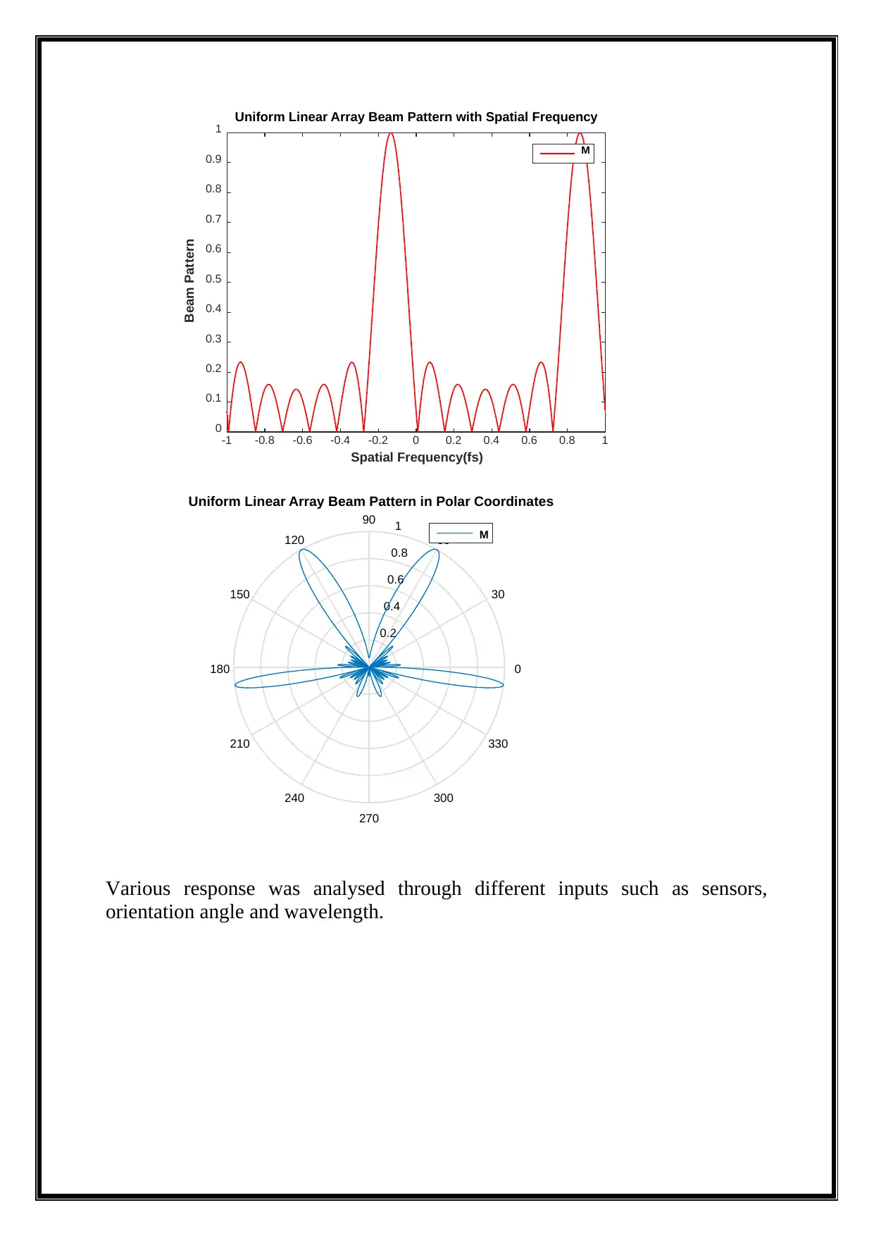
Uniform Linear Array Beam Pattern with Spatial Frequency
M
0.2
0.4
0.6
0.8
1
30
210
60
240
90
270
120
300
150
330
180 0
Uniform Linear Array Beam Pattern in Polar Coordinates
M
Various response was analysed through different inputs such as sensors,
orientation angle and wavelength.
-1 -0.8 -0.6 -0.4 -0.2 0 0.2 0.4 0.6 0.8 1
Beam Pattern
0
0.1
0.2
0.3
0.4
0.5
0.6
0.7
0.8
0.9
1
Uniform Linear Array Beam Pattern with Spatial Frequency
M
0.2
0.4
0.6
0.8
1
30
210
60
240
90
270
120
300
150
330
180 0
Uniform Linear Array Beam Pattern in Polar Coordinates
M
Various response was analysed through different inputs such as sensors,
orientation angle and wavelength.
1 out of 18
Your All-in-One AI-Powered Toolkit for Academic Success.
+13062052269
info@desklib.com
Available 24*7 on WhatsApp / Email
![[object Object]](/_next/static/media/star-bottom.7253800d.svg)
Unlock your academic potential
© 2024 | Zucol Services PVT LTD | All rights reserved.