Random Variables With Joint Probability PDF 2022

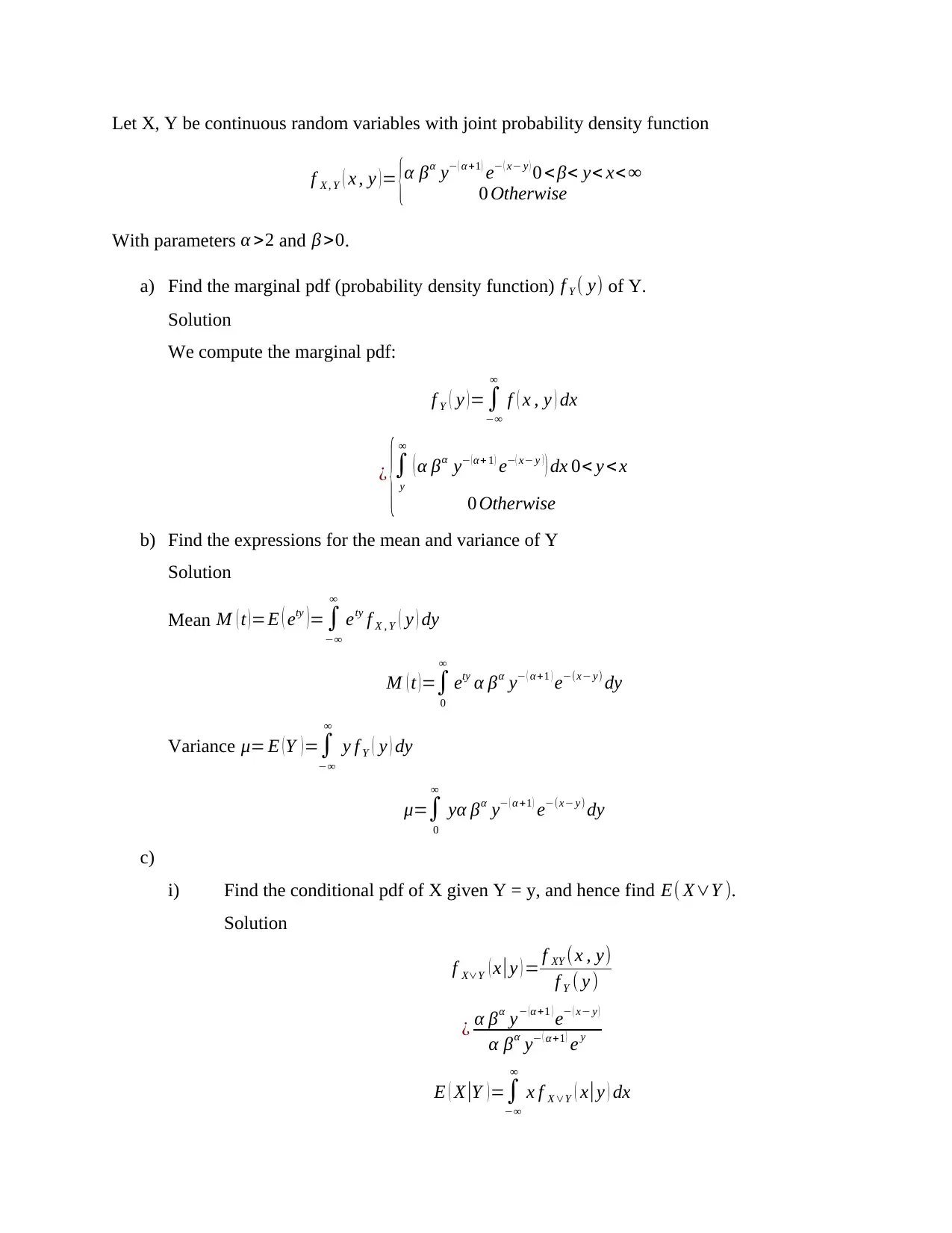
Let X, Y be continuous random variables with joint probability density function
f X , Y ( x , y ) = {α βα y− ( α +1 ) e− ( x− y ) 0 <β< y< x< ∞
0 Otherwise
With parameters α >2 and β >0.
a) Find the marginal pdf (probability density function) f Y ( y) of Y.
Solution
We compute the marginal pdf:
f Y ( y ) =∫
−∞
∞
f ( x , y ) dx
¿
{∫
y
∞
( α βα y− (α+ 1 ) e−( x− y ) ) dx 0< y < x
0 Otherwise
b) Find the expressions for the mean and variance of Y
Solution
Mean M ( t )=E ( ety )=∫
−∞
∞
ety f X , Y ( y ) dy
M ( t ) =∫
0
∞
ety α βα y− ( α +1 ) e−(x− y) dy
Variance μ= E (Y )=∫
−∞
∞
y f Y ( y ) dy
μ=∫
0
∞
yα βα y− ( α +1 ) e−(x− y) dy
c)
i) Find the conditional pdf of X given Y = y, and hence find E( X∨Y ).
Solution
f X∨Y ( x|y ) = f XY (x , y)
f Y ( y )
¿ α βα y− (α+1 ) e− ( x− y )
α βα y− ( α+1 ) e y
E ( X |Y ) =∫
−∞
∞
x f X ∨Y ( x| y ) dx

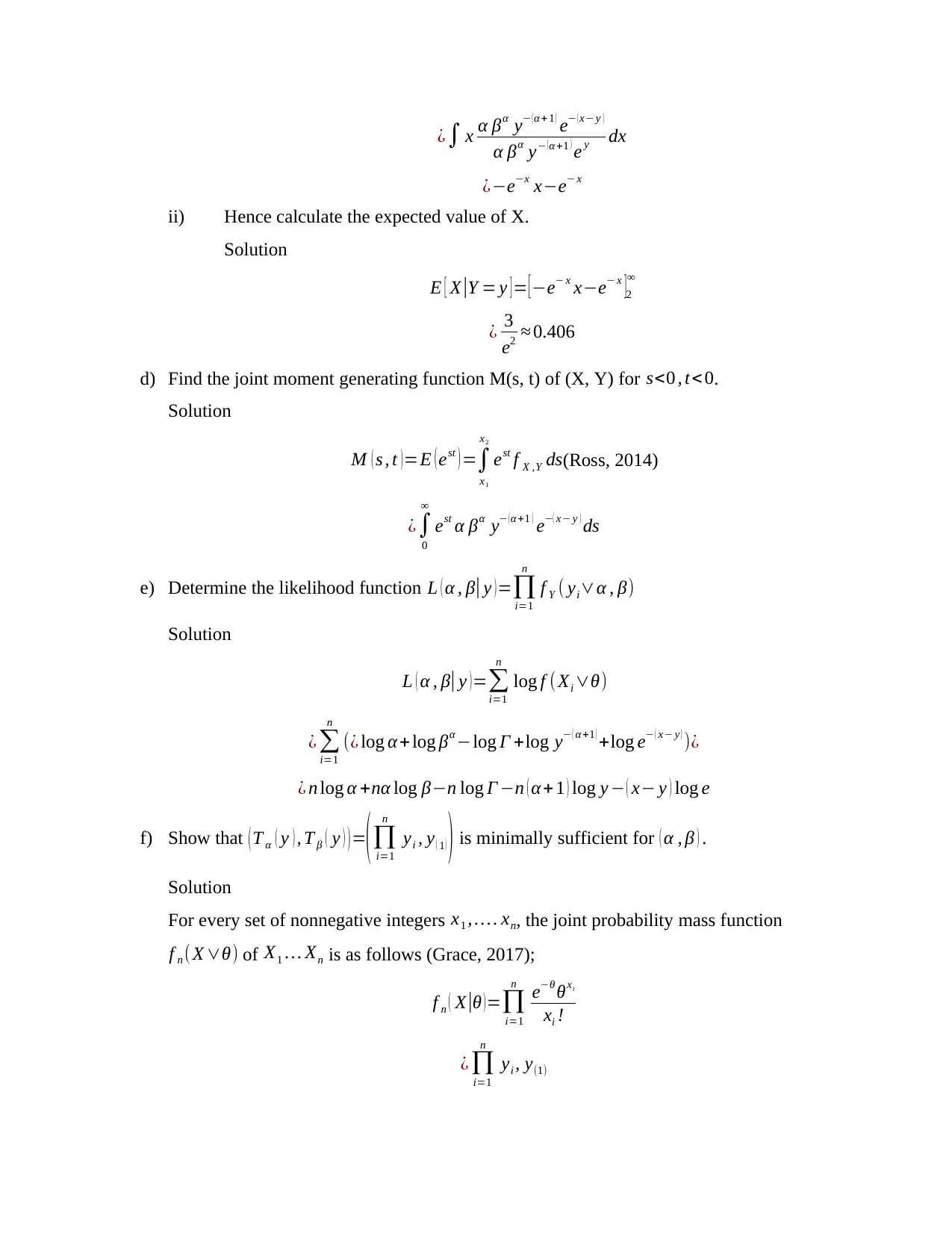
¿∫ x α βα y− ( α+ 1 ) e− ( x− y )
α βα y− ( α +1 ) e y dx
¿−e−x x−e− x
ii) Hence calculate the expected value of X.
Solution
E [ X |Y = y ] = [ −e− x x−e− x ]2
∞
¿ 3
e2 ≈ 0.406
d) Find the joint moment generating function M(s, t) of (X, Y) for s<0 , t<0.
Solution
M ( s , t )=E ( est ) =∫
x1
x2
est f X ,Y ds(Ross, 2014)
¿∫
0
∞
est α βα y− ( α+1 ) e−( x− y ) ds
e) Determine the likelihood function L ( α , β|y )=∏
i=1
n
f Y ( yi∨α , β)
Solution
L ( α , β| y ) =∑
i=1
n
log f ( Xi ∨θ)
¿ ∑
i=1
n
(¿ log α + log βα−log Γ +log y− ( α +1 ) +log e− ( x− y ) )¿
¿ n log α +nα log β−n log Γ −n ( α + 1 ) log y − ( x− y ) log e
f) Show that ( T α ( y ) , T β ( y ) ) =
( ∏
i=1
n
yi , y ( 1 ) ) is minimally sufficient for ( α , β ) .
Solution
For every set of nonnegative integers x1 , … . xn, the joint probability mass function
f n ( X ∨θ) of X1 … Xn is as follows (Grace, 2017);
f n ( X |θ ) =∏
i=1
n e−θ θxi
xi !
¿ ∏
i=1
n
yi , y(1)

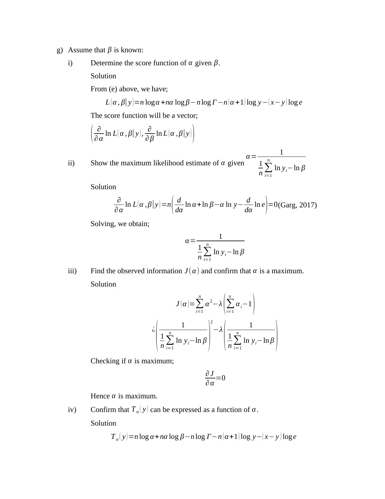
g) Assume that β is known:
i) Determine the score function of α given β.
Solution
From (e) above, we have;
L ( α , β|y )=n logα +nα log β−n log Γ −n ( α +1 ) log y − ( x− y ) log e
The score function will be a vector;
( ∂
∂ α ln L ( α , β| y ) , ∂
∂ β ln L ( α , β | y ) )
ii) Show the maximum likelihood estimate of α given α = 1
1
n ∑
i=1
n
ln yi−ln β
Solution
∂
∂ α ln L ( α , β |y ) =n ( d
dα ln α+ ln β−α ln y− d
dα ln e )=0(Garg, 2017)
Solving, we obtain;
α= 1
1
n ∑
i=1
n
ln yi−ln β
iii) Find the observed information J ( α) and confirm that α is a maximum.
Solution
J ( α ) =∑
i=1
n
α 2−λ ( ∑
i=1
n
α i−1 )
¿
( 1
1
n ∑
i=1
n
ln yi−ln β )
2
−λ
( 1
1
n ∑
i=1
n
ln yi−ln β )
Checking if α is maximum;
∂ J
∂ α =0
Hence α is maximum.
iv) Confirm that T α ( y ) can be expressed as a function of α .
Solution
T α ( y ) =n log α +nα log β−n log Γ−n ( α +1 ) log y− ( x− y ) log e

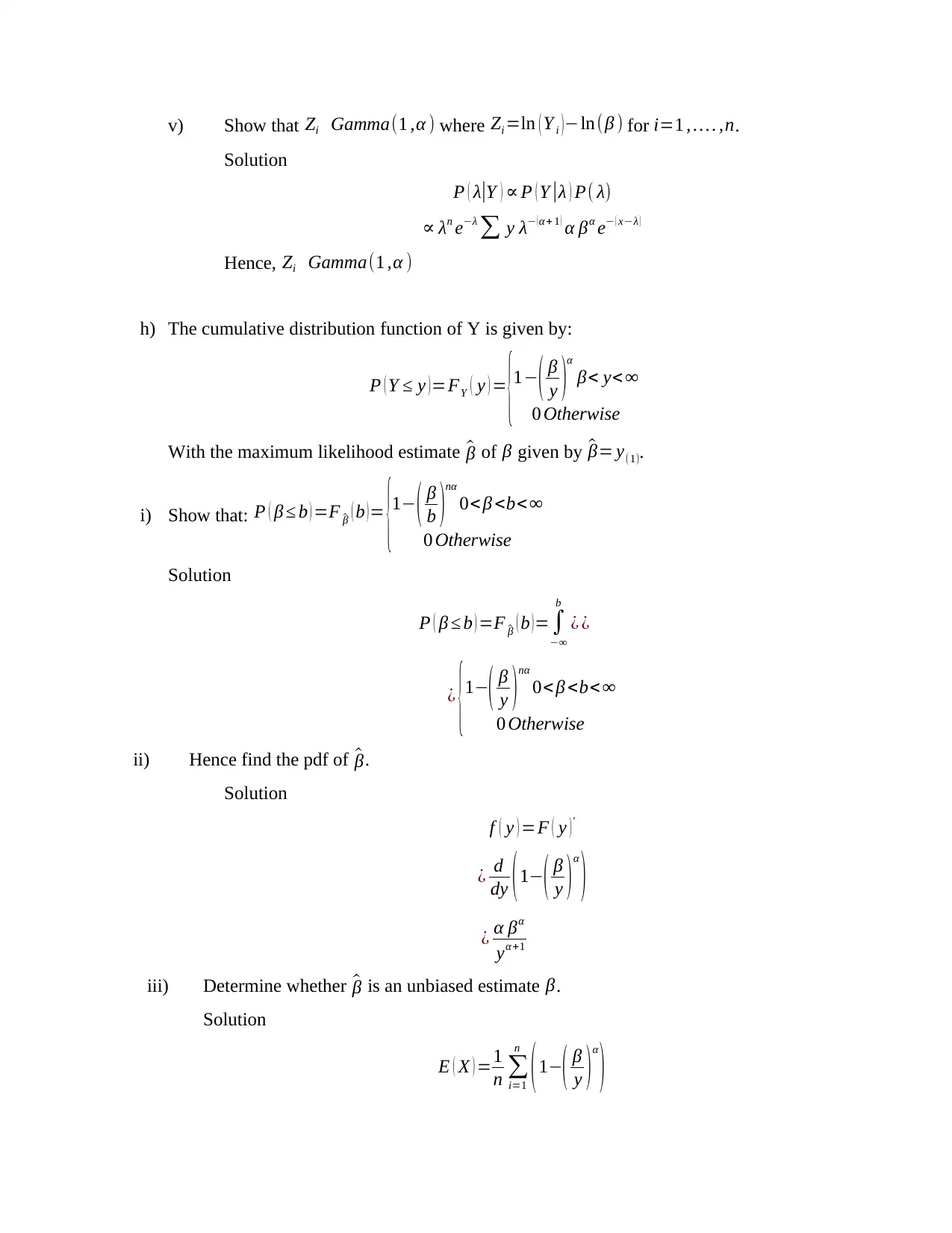
v) Show that Zi Gamma(1 ,α ) where Zi =ln ( Y i )−ln(β ) for i=1 , … . ,n.
Solution
P ( λ|Y ) ∝ P ( Y |λ ) P( λ)
∝ λn e−λ
∑ y λ− (α+ 1 ) α βα e− ( x−λ )
Hence, Zi Gamma(1 ,α )
h) The cumulative distribution function of Y is given by:
P ( Y ≤ y )=FY ( y ) =
{1−( β
y )α
β< y< ∞
0 Otherwise
With the maximum likelihood estimate ^β of β given by ^β= y(1).
i) Show that: P ( β ≤ b ) =F ^β ( b ) = {1− ( β
b )
nα
0< β <b< ∞
0 Otherwise
Solution
P ( β ≤ b ) =F ^β ( b ) =∫
−∞
b
¿ ¿
¿
{1−( β
y ) nα
0< β <b< ∞
0 Otherwise
ii) Hence find the pdf of ^β.
Solution
f ( y ) =F ( y )'
¿ d
dy ( 1−( β
y ) α
)
¿ α βα
yα+1
iii) Determine whether ^β is an unbiased estimate β.
Solution
E ( X ) =1
n ∑
i=1
n
(1−( β
y )α
)

¿ 1− ( β
y )
α
Thus, ^β is an unbiased estimate β.
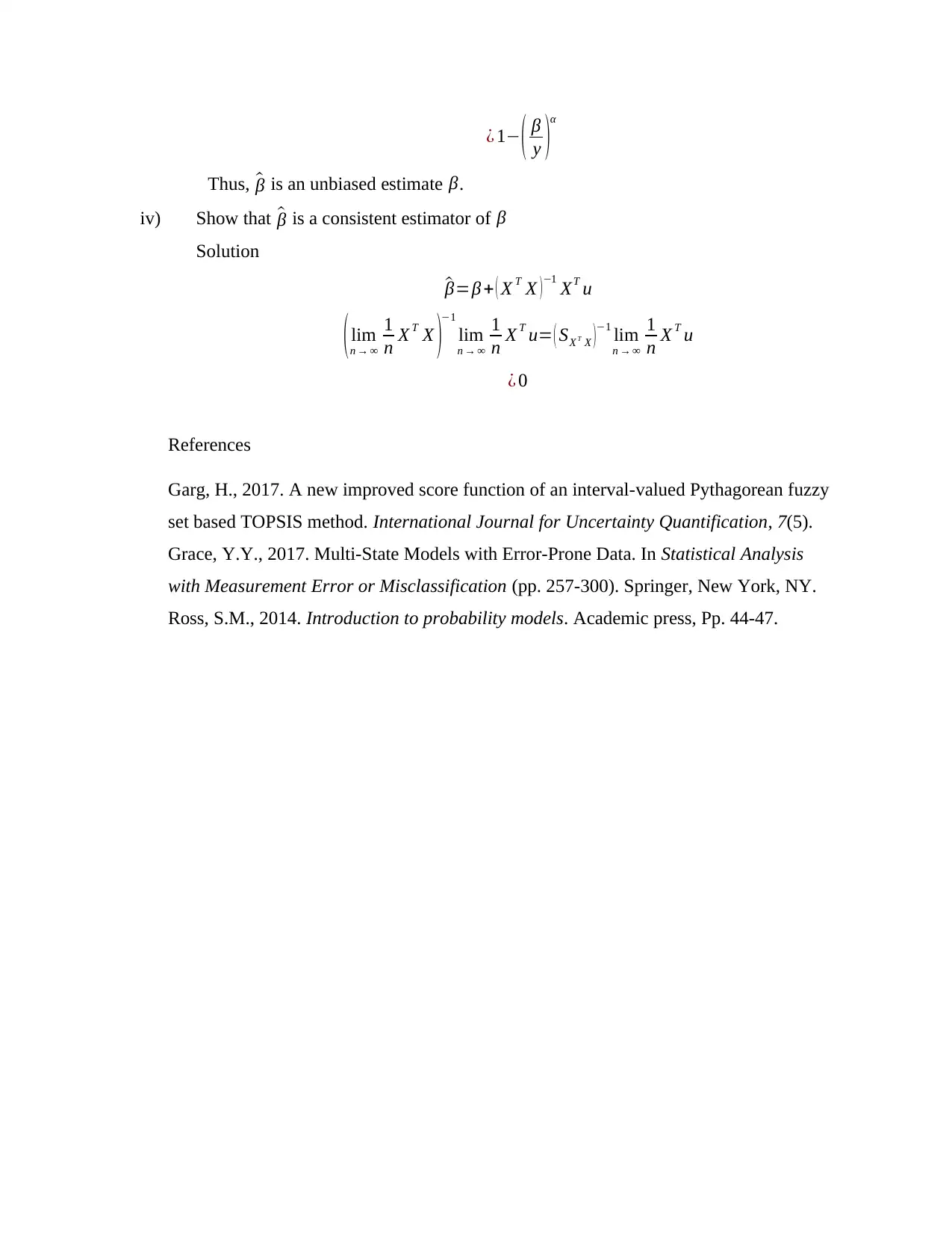
iv) Show that ^β is a consistent estimator of β
Solution
^β=β + ( X T X )−1
XT u
(lim
n → ∞
1
n X T X )−1
lim
n → ∞
1
n X T u= ( SX T X )−1 lim
n → ∞
1
n X T u
¿ 0
References
Garg, H., 2017. A new improved score function of an interval-valued Pythagorean fuzzy
set based TOPSIS method. International Journal for Uncertainty Quantification, 7(5).
Grace, Y.Y., 2017. Multi-State Models with Error-Prone Data. In Statistical Analysis
with Measurement Error or Misclassification (pp. 257-300). Springer, New York, NY.
Ross, S.M., 2014. Introduction to probability models. Academic press, Pp. 44-47.