Regression Analysis

Running head: REGRESSION ANALYSIS
REGRESSION ANALYSIS
Name of the Student
Name of the University
Author Note

1REGRESSION ANALYSIS
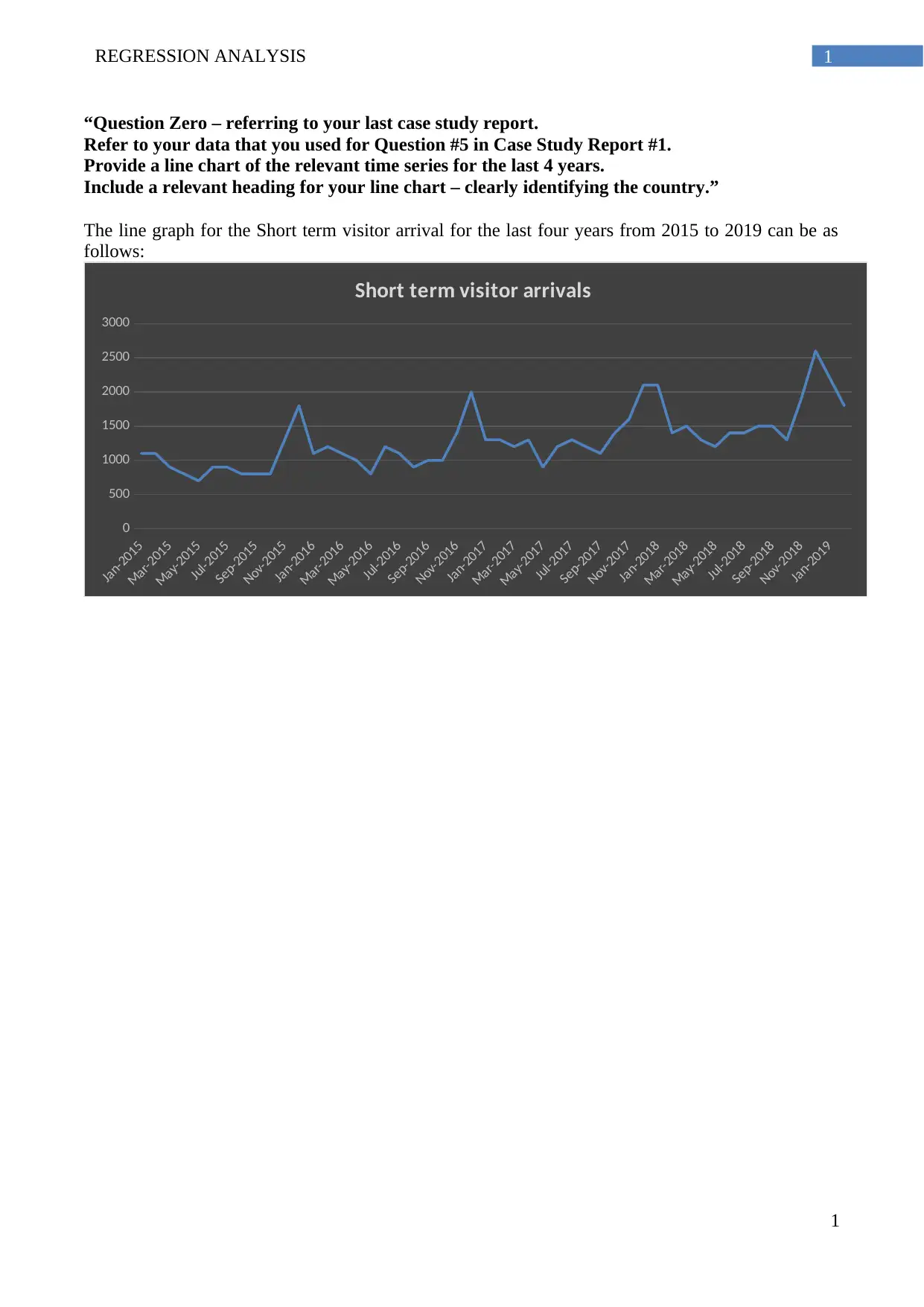
“Question Zero – referring to your last case study report.
Refer to your data that you used for Question #5 in Case Study Report #1.
Provide a line chart of the relevant time series for the last 4 years.
Include a relevant heading for your line chart – clearly identifying the country.”
The line graph for the Short term visitor arrival for the last four years from 2015 to 2019 can be as
follows:
Jan-2015
Mar-2015
May-2015
Jul-2015
Sep-2015
Nov-2015
Jan-2016
Mar-2016
May-2016
Jul-2016
Sep-2016
Nov-2016
Jan-2017
Mar-2017
May-2017
Jul-2017
Sep-2017
Nov-2017
Jan-2018
Mar-2018
May-2018
Jul-2018
Sep-2018
Nov-2018
Jan-2019
0
500
1000
1500
2000
2500
3000
Short term visitor arrivals
1

2REGRESSION ANALYSIS
Q1. “Estimate the parameters of a multiple linear regression model for visitor arrivals using an
intercept, a time variable and a suitable set of dummy variables for the month effect. Explain
what you have done, provide relevant screenshots, and write out the overall regression
equation.”
In order to find out the visitor arrival and find a multiple linear regression model for the
visitor arrival by making use of an intercept, the following parameters have to be determined:
Time variable
The time variable which has been chosen for the purpose of analysis can be understood t0 be
from the period March 2018 to 2019. This will help in ensuring that the latest trends are estimated
and that the visitors present in the country can be estimates successfully (Harrell Jr 2015).
Dummy variables
The dummy variables which have been chosen for the purpose of the years were made use of
is if analysis and they were written down in numbers (Carroll 2017).
dummy1 dumm2 y x x2 xy
Feb-2017 2 1 1300 0 0 0
Mar-2017 3 1 1200 1 1 3
Apr-2017 4 1 1300 2 4 16
May-2017 5 1 900 3 9 45
Jun-2017 6 1 1200 4 16 96
Jul-2017 7 1 1300 5 25 175
Aug-2017 8 1 1200 6 36 288
Sep-2017 9 1 1100 7 49 441
Oct-2017 10 1 1400 8 64 640
Nov-2017 11 1 1600 9 81 891
Dec-2017 12 1 2100 10 100 1200
Jan-2018 1 2 2100 -1 1 1
Feb-2018 2 2 1400 0 0 0
Mar-2018 3 2 1500 1 1 3
Apr-2018 4 2 1300 2 4 16
May-2018 5 2 1200 3 9 45
Jun-2018 6 2 1400 4 16 96
Jul-2018 7 2 1400 5 25 175
Aug-2018 8 2 1500 6 36 288
Sep-2018 9 2 1500 7 49 441
Oct-2018 10 2 1300 8 64 640
Nov-2018 11 2 1900 9 81 891
Dec-2018 12 2 2600 10 100 1200
Jan-2019 1 3 2200 -1 1 1
Feb-2019 2 3 1800 0 0 0
158 37700 108 772 7592
Intercept
2

3REGRESSION ANALYSIS
The value of the x be taken to be as 1 as it helps to understand the overall values of the
different years and the difference between the dummy variables chosen to replace the month and the
years
In order to ensure that two dummy variables were chosen for multiple linear regression model. A
total of 25 data sets were chosen which began from February 2017 to February 2019. Hence, in line
of this, the months were given a dummy variable of numbers 1 to 12 and the years were also labelled
accordingly from 1. These helped in figuring out the overall trend and the regression line as well.
Therefore, when the regression was carried out, the following data was received as a result:
Coefficie
nts
Standar
d Error t Stat P-value
Lower
95%
Upper
95%
Lower
95.0%
Upper
95.0%
Interce
pt 572.8261
296.07
9
1.9347
07
0.0666
11
-
42.903
9
1188.5
56
-
42.903
9
1188.5
56
2 43.47826
21.831
47
1.9915
4
0.0595
87
-
1.9227
7
88.879
29
-
1.9227
7
88.879
29
1 396.7391
120.85
03
3.2828
98
0.0035
49
145.41
72
648.06
1
145.41
72
648.06
1
This means that the regression line is
Y=572.82+43.47(YEAR) +396.7(Month)
Hence, the intercept is 572.82 approximately
Q2. “Explain the meaning of the intercept, the coefficient of the time variable, as well as the
coefficient for the June dummy variable. (If June is your baseline, then change June to
September).”
 Intercept: In such a scenario, the intercept can be understood to be relatively stable in nature
and hence, it reflects that the intercept can be stated to have a major influence on the Y
variable. The intercept can be understood to be the expected mean value of Y in case X is
considered to be 0 (Darlington and Hayes 2016). Very often when X=0 then the intercept is
the expected mean of the Y value.
 Coefficient of time variable: The coefficient of the time variable in such a scenario tends to
take into consideration the time gap which exists between the given time range. In such a
case the time variable has been taken to be a gap of one month which predicts the customer in
take every period (Fox 2015).
 Coefficient for the June dummy variable: The coefficient of June variable can be understood
to be moderate in nature which reflects that the customer intake is maximum in this given
period of time (Chatterjee and Hadi 2015).

3

References

Breiman, L., 2017. Classification and regression trees. Routledge.
Carroll, R.J., 2017. Transformation and weighting in regression. Routledg
Chatterjee, S. and Hadi, A.S., 2015. Regression analysis by example. John Wiley & Sons.
Cohen, P., West, S.G. and Aiken, L.S., 2014. Applied multiple regression/correlation analysis for the
behavioral sciences. Psychology Press.
Darlington, R.B. and Hayes, A.F., 2016. Regression analysis and linear models: Concepts,
applications, and implementation. Guilford Publications.
Fox, J., 2015. Applied regression analysis and generalized linear models. Sage Publications.
Harrell Jr, F.E., 2015. Regression modeling strategies: with applications to linear models, logistic
and ordinal regression, and survival analysis. Springer.
Hayes, A.F., 2017. Introduction to mediation, moderation, and conditional process analysis: A
regression-based approach. Guilford Publications.
Hoffmann, J.P. and Shafer, K., 2015. Linear regression analysis. Washington, DC: NASW Press.
Hox, J.J., Moerbeek, M. and Van de Schoot, R., 2017. Multilevel analysis: Techniques and
applications. Routledge.
Sagoe, D., Molde, H., Andreassen, C.S., Torsheim, T. and Pallesen, S., 2014. The global
epidemiology of anabolic-androgenic steroid use: a meta-analysis and meta-regression
analysis. Annals of epidemiology, 24(5), pp.383-398.
Schroeder, L.D., Sjoquist, D.L. and Stephan, P.E., 2016. Understanding regression analysis: An
introductory guide (Vol. 57). Sage Publications.
Sperandei, S., 2014. Understanding logistic regression analysis. Biochemia medica: Biochemia
medica, 24(1), pp.12-18.
9
Paraphrase This Document
Need a fresh take? Get an instant paraphrase of this document with our AI Paraphraser