Regression Analysis of Production and Sales: BIT435 Report

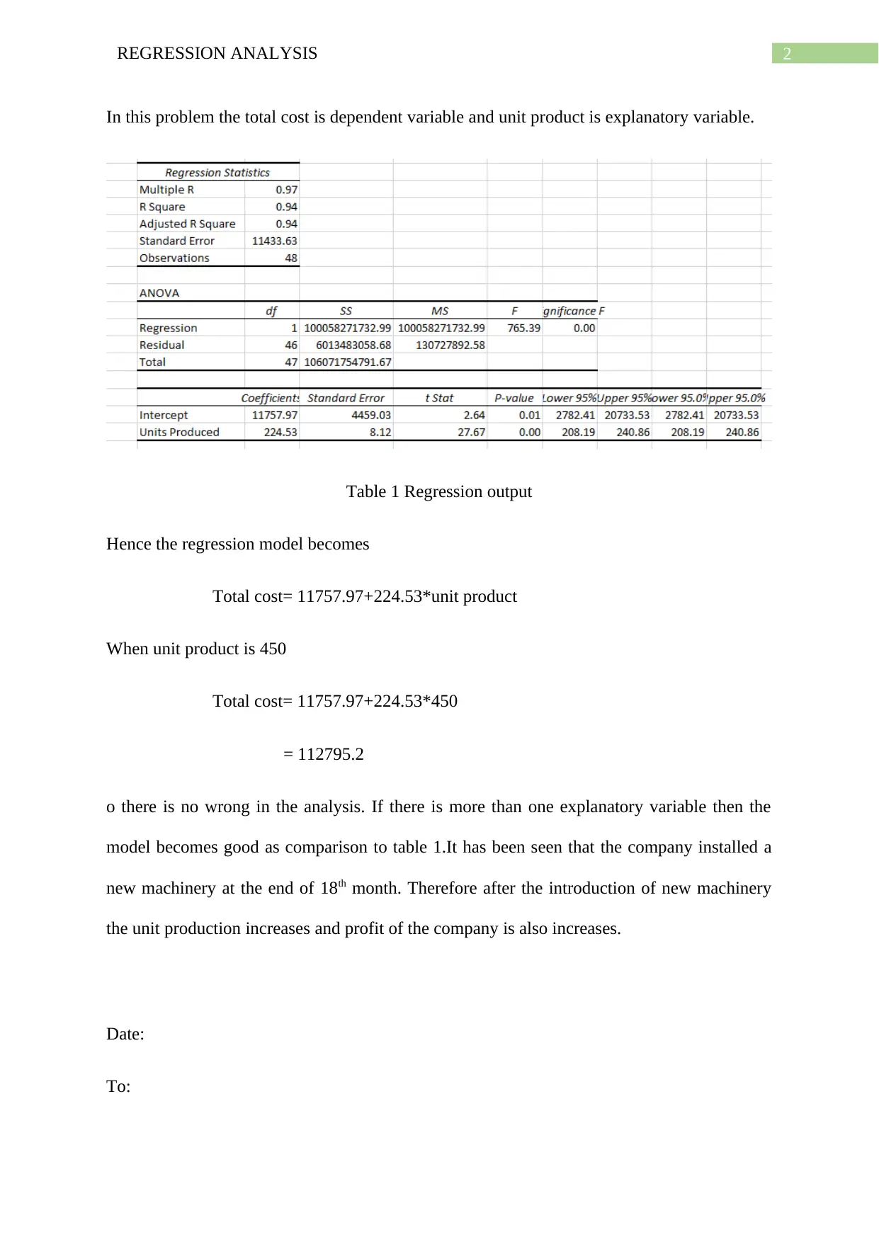
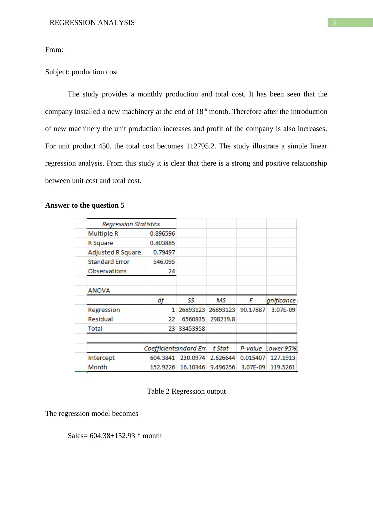
This report provides a comprehensive analysis of several regression problems. It begins by examining the relationship between production levels and total costs, using simple linear regression to predict future costs and discusses the limitations of the initial model, suggesting modifications to account...Read More

Running head: REGRESSION ANALYSIS
Regression Analysis
Name of the Student:
Name of the University:
Author note:

1REGRESSION ANALYSIS
Table of Contents
Answer to the question 3............................................................................................................2
Answer to the question 5............................................................................................................3
Answer to the question 6............................................................................................................4
Answer to the question 11..........................................................................................................5
Part (a)....................................................................................................................................5
Part (b)....................................................................................................................................5
Part (c)....................................................................................................................................6
Answer to the question 12..........................................................................................................7
Answer to the question 17..........................................................................................................8
Part (a)....................................................................................................................................8
Part (b)....................................................................................................................................8
Part (c)....................................................................................................................................9
Bibliography.............................................................................................................................11
Answer to the question 3

2REGRESSION ANALYSIS
In this problem the total cost is dependent variable and unit product is explanatory variable.
Table 1 Regression output
Hence the regression model becomes
Total cost= 11757.97+224.53*unit product
When unit product is 450
Total cost= 11757.97+224.53*450
= 112795.2
o there is no wrong in the analysis. If there is more than one explanatory variable then the
model becomes good as comparison to table 1.It has been seen that the company installed a
new machinery at the end of 18th month. Therefore after the introduction of new machinery
the unit production increases and profit of the company is also increases.
Date:
To:

3REGRESSION ANALYSIS
From:
Subject: production cost
The study provides a monthly production and total cost. It has been seen that the
company installed a new machinery at the end of 18th month. Therefore after the introduction
of new machinery the unit production increases and profit of the company is also increases.
For unit product 450, the total cost becomes 112795.2. The study illustrate a simple linear
regression analysis. From this study it is clear that there is a strong and positive relationship
between unit cost and total cost.
Answer to the question 5
Table 2 Regression output
The regression model becomes
Sales= 604.38+152.93 * month

4REGRESSION ANALYSIS
0 5 10 15 20 25 30
0
500
1000
1500
2000
2500
3000
3500
4000
Scatter Plot
Month
Sales
Figure 1 Scatter plot on Month versus sales
Figure 1 shows relationship between months versus sales. In the X-axis represent the
months and Y-axis represent the sales. During the period of 24 months the sales is linearly
distributed among the month. With the help of trend line this can easily defined. The sales
data is lies entire the trend or diagonal line.
Answer to the question 6

5REGRESSION ANALYSIS
Table 3 Regression output
The regression equation becomes
Price= 63745.15+49.37* Home size
The value of the R- square is 0.49.
The standard error of the estimate is 29945.59.
Answer to the question 11
Part (a)
It is expected that the sign of the explanatory variable is positive. The explanatory
variable of this study are price per ride, population, income and parking rate. Moreover in
riding it is expected that the study variable should be significant and positive. The price for
ride always increases, population is also increases. The income and parking rate is depends
upon the situation.
Part (b)

6REGRESSION ANALYSIS
Table 3 Regression output
The multiple linear regression equation becomes
Weekly riders= 124.43+ (-166.96)*price ride+0.62* population+ (-0.05)*income+194.68 *
parking rate.
The coefficient of this regression analysis are as below
Price ride= -166.96
Population= 0.62
Income = -0.05
Parking rate= 194.68
Yes. But the coefficient of price on ride is surprising. Because it is highly negative.
Moreover the other variable income is also negative.
Part (c)
Year or time is not mentioned in this multiple regression analysis.

7REGRESSION ANALYSIS
Answer to the question 12
Table 4 Regression output
The regression model becomes
Total production cost= 4642.56+63.21*unit of product 1+32.57*unit of product 2+58.82*unit
of product 3+26.23* unit of product 4
To calculate the fixed cost the variable cost is needed. Because total cost is the sum of
fixed and variable cost. Yes with the help of fixed and variable cost the total cost can be
easily determined.

8REGRESSION ANALYSIS
Answer to the question 17
Part (a)
Table 5 Regression output (model 1)
The simple linear regression model is as below
Annual sales= 8038.48+0.07* population
The value of the R-square is 0.02.
Part (b)

9REGRESSION ANALYSIS
Table 6 Regression output (model 2)
After adding one new explanatory the multiple linear regression becomes
Annual sales= 4279.08+0.07*population+0.16*advertising
The value of R-square is 0.29. It is higher than the simple linear regression R-square
value. Hence it is a better model as compared to simple linear regression model.
In model 1 the value of the adjusted R-square is -0.04 and in model 2 it is 0.20. Thus
in model 1 that is in simple linear regression model adjusted is very low and it going to reach
at negativity. But the model 2 shows a positive sense in adjusted R-square.
Part (c)
Table 7 Regression output (model 3)
Again after adding new variable the regression model becomes
Annual sales = -4770.20+0.10*population+0.12* advertising+0.27* previous advertisement

10REGRESSION ANALYSIS
In the new model the value of the R-square is 0.99. Which is very high and going to
reach at perfect positive relation. As compared to model 2 the R-square value of model is
strong and better.

11REGRESSION ANALYSIS
Bibliography
Cameron, A. C., & Trivedi, P. K. (2013). Regression analysis of count data (Vol. 53).
Cambridge university press.
Chatterjee, S., & Hadi, A. S. (2015). Regression analysis by example. John Wiley & Sons.
Kleinbaum, D. G., Kupper, L. L., Nizam, A., & Rosenberg, E. S. (2013). Applied regression
analysis and other multivariable methods. Nelson Education.
Sperandei, S. (2014). Understanding logistic regression analysis. Biochemia medica:
Biochemia medica, 24(1), 12-18.