
1
ECON 5313: Decisions and Strategies
Module 3 HW: Estimating a Regression
ECON 5313: Decisions and Strategies
Module 3 HW: Estimating a Regression
Paraphrase This Document
Need a fresh take? Get an instant paraphrase of this document with our AI Paraphraser
2
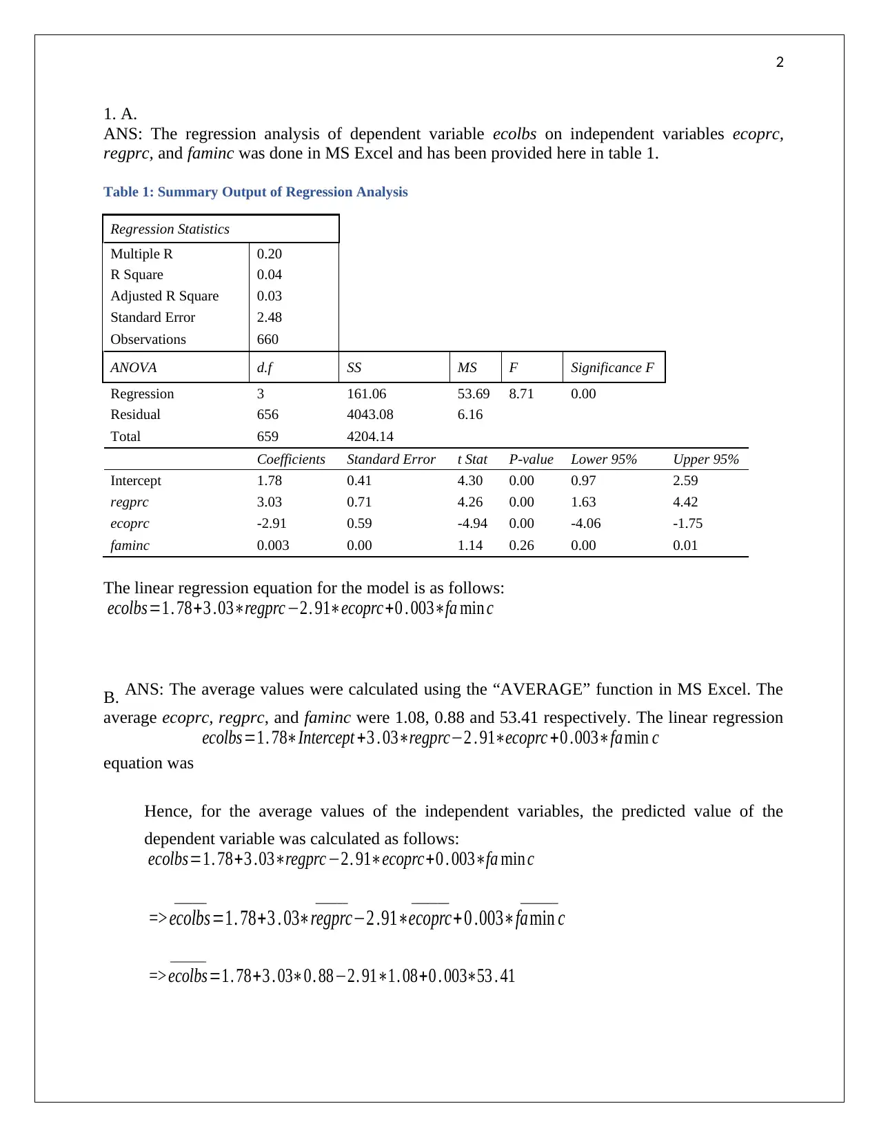
1. A.
ANS: The regression analysis of dependent variable ecolbs on independent variables ecoprc,
regprc, and faminc was done in MS Excel and has been provided here in table 1.
Table 1: Summary Output of Regression Analysis
Regression Statistics
Multiple R 0.20
R Square 0.04
Adjusted R Square 0.03
Standard Error 2.48
Observations 660
ANOVA d.f SS MS F Significance F
Regression 3 161.06 53.69 8.71 0.00
Residual 656 4043.08 6.16
Total 659 4204.14
Coefficients Standard Error t Stat P-value Lower 95% Upper 95%
Intercept 1.78 0.41 4.30 0.00 0.97 2.59
regprc 3.03 0.71 4.26 0.00 1.63 4.42
ecoprc -2.91 0.59 -4.94 0.00 -4.06 -1.75
faminc 0.003 0.00 1.14 0.26 0.00 0.01
The linear regression equation for the model is as follows:
ecolbs=1. 78+3 .03∗regprc −2. 91∗ecoprc+0 . 003∗fa min c
B. ANS: The average values were calculated using the “AVERAGE” function in MS Excel. The
average ecoprc, regprc, and faminc were 1.08, 0.88 and 53.41 respectively. The linear regression
equation was
ecolbs=1. 78∗Intercept +3 . 03∗regprc−2 . 91∗ecoprc +0 .003∗famin c
Hence, for the average values of the independent variables, the predicted value of the
dependent variable was calculated as follows:
ecolbs=1. 78+3 .03∗regprc −2. 91∗ecoprc+0 . 003∗fa min c
=> ecolbs
______
=1. 78+3 . 03∗regprc
______
−2 .91∗ecoprc
_______
+ 0 .003∗famin c
_______
=> ecolbs
_______
=1. 78+3 . 03∗0. 88−2. 91∗1. 08+0 . 003∗53 . 41
3
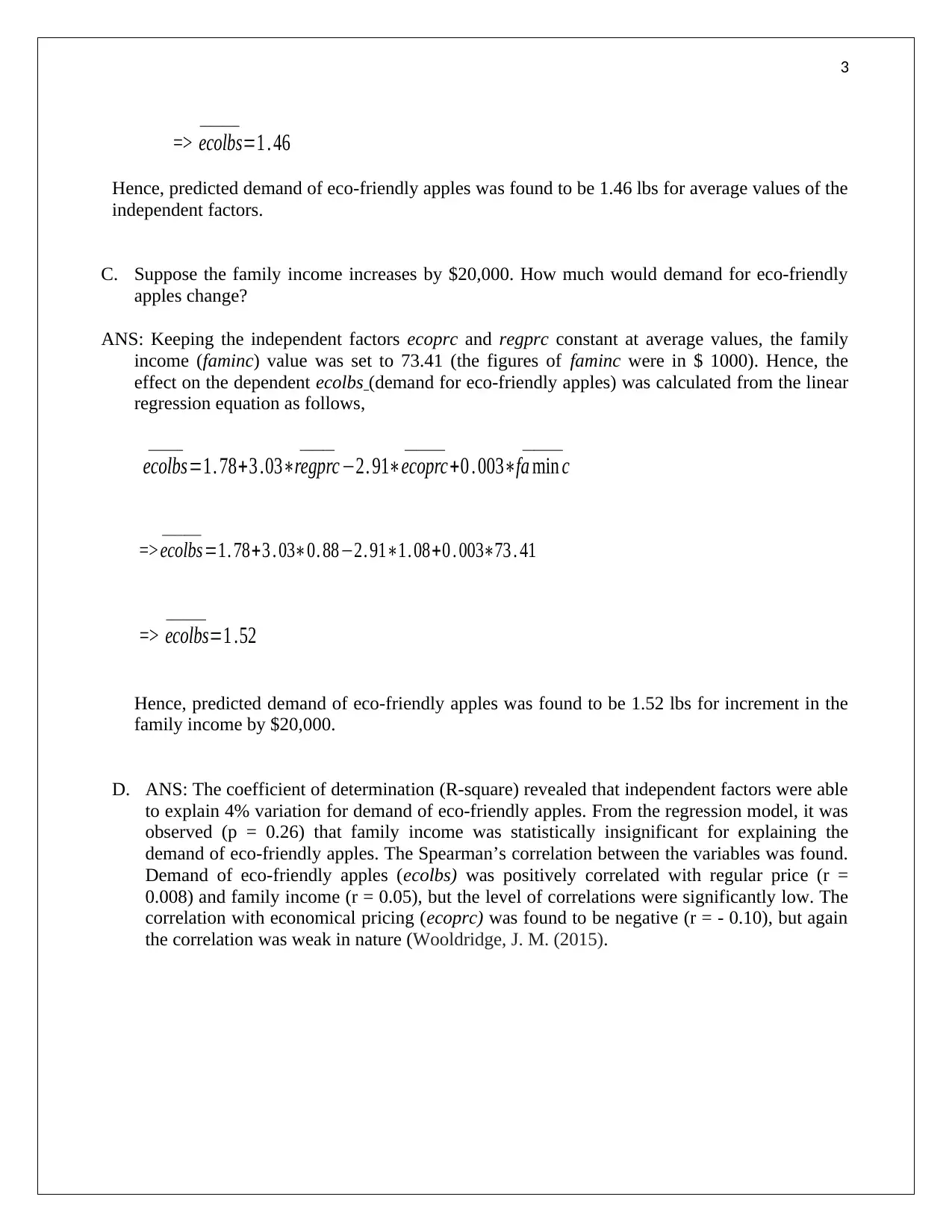
=> ecolbs
_______
=1 . 46
Hence, predicted demand of eco-friendly apples was found to be 1.46 lbs for average values of the
independent factors.
C. Suppose the family income increases by $20,000. How much would demand for eco-friendly
apples change?
ANS: Keeping the independent factors ecoprc and regprc constant at average values, the family
income (faminc) value was set to 73.41 (the figures of faminc were in $ 1000). Hence, the
effect on the dependent ecolbs (demand for eco-friendly apples) was calculated from the linear
regression equation as follows,
ecolbs
______
=1. 78+3 .03∗regprc
______
−2. 91∗ecoprc
_______
+0 . 003∗fa min c
_______
=> ecolbs
_______
=1. 78+3 . 03∗0. 88−2. 91∗1. 08+0 . 003∗73 . 41
=> ecolbs
_______
=1 .52
Hence, predicted demand of eco-friendly apples was found to be 1.52 lbs for increment in the
family income by $20,000.
D. ANS: The coefficient of determination (R-square) revealed that independent factors were able
to explain 4% variation for demand of eco-friendly apples. From the regression model, it was
observed (p = 0.26) that family income was statistically insignificant for explaining the
demand of eco-friendly apples. The Spearman’s correlation between the variables was found.
Demand of eco-friendly apples (ecolbs) was positively correlated with regular price (r =
0.008) and family income (r = 0.05), but the level of correlations were significantly low. The
correlation with economical pricing (ecoprc) was found to be negative (r = - 0.10), but again
the correlation was weak in nature (Wooldridge, J. M. (2015).
=> ecolbs
_______
=1 . 46
Hence, predicted demand of eco-friendly apples was found to be 1.46 lbs for average values of the
independent factors.
C. Suppose the family income increases by $20,000. How much would demand for eco-friendly
apples change?
ANS: Keeping the independent factors ecoprc and regprc constant at average values, the family
income (faminc) value was set to 73.41 (the figures of faminc were in $ 1000). Hence, the
effect on the dependent ecolbs (demand for eco-friendly apples) was calculated from the linear
regression equation as follows,
ecolbs
______
=1. 78+3 .03∗regprc
______
−2. 91∗ecoprc
_______
+0 . 003∗fa min c
_______
=> ecolbs
_______
=1. 78+3 . 03∗0. 88−2. 91∗1. 08+0 . 003∗73 . 41
=> ecolbs
_______
=1 .52
Hence, predicted demand of eco-friendly apples was found to be 1.52 lbs for increment in the
family income by $20,000.
D. ANS: The coefficient of determination (R-square) revealed that independent factors were able
to explain 4% variation for demand of eco-friendly apples. From the regression model, it was
observed (p = 0.26) that family income was statistically insignificant for explaining the
demand of eco-friendly apples. The Spearman’s correlation between the variables was found.
Demand of eco-friendly apples (ecolbs) was positively correlated with regular price (r =
0.008) and family income (r = 0.05), but the level of correlations were significantly low. The
correlation with economical pricing (ecoprc) was found to be negative (r = - 0.10), but again
the correlation was weak in nature (Wooldridge, J. M. (2015).
⊘ This is a preview!⊘
Do you want full access?
Subscribe today to unlock all pages.
Trusted by 1+ million students worldwide
4
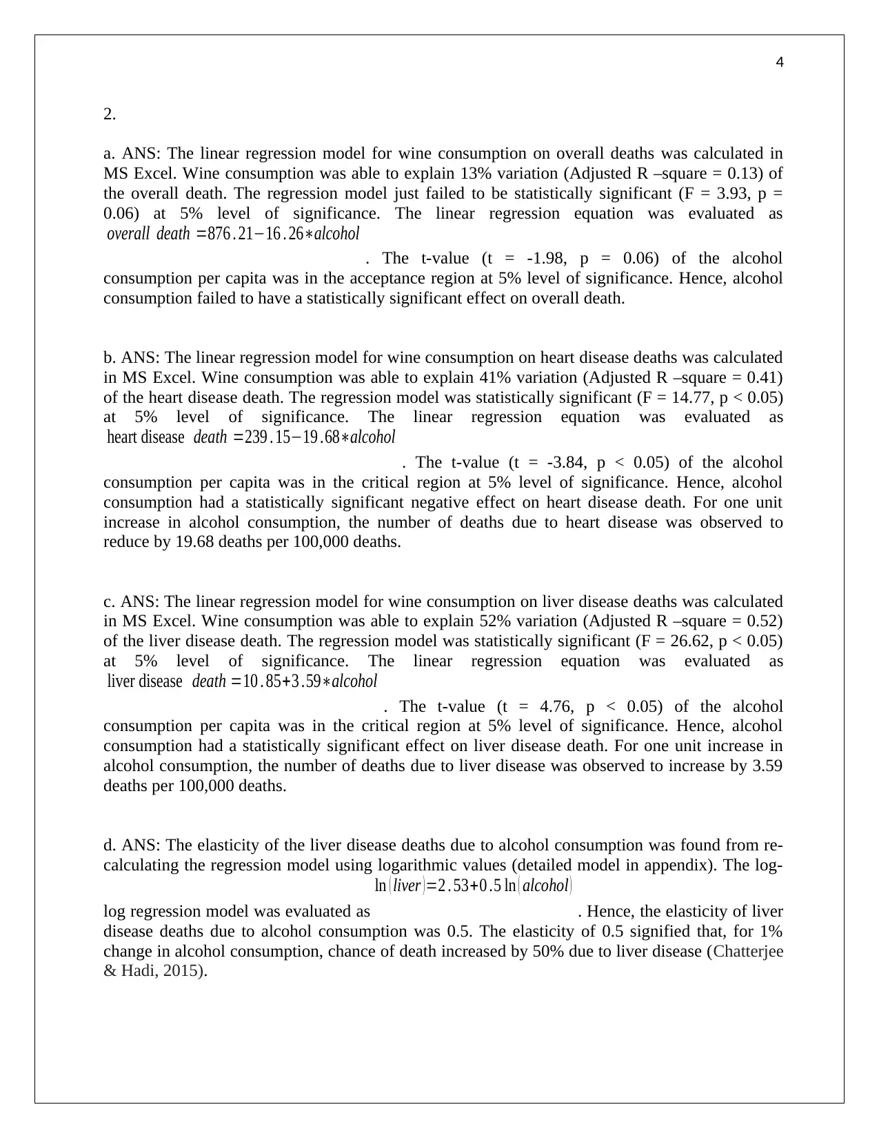
2.
a. ANS: The linear regression model for wine consumption on overall deaths was calculated in
MS Excel. Wine consumption was able to explain 13% variation (Adjusted R –square = 0.13) of
the overall death. The regression model just failed to be statistically significant (F = 3.93, p =
0.06) at 5% level of significance. The linear regression equation was evaluated as
overall death =876 . 21−16 . 26∗alcohol
. The t-value (t = -1.98, p = 0.06) of the alcohol
consumption per capita was in the acceptance region at 5% level of significance. Hence, alcohol
consumption failed to have a statistically significant effect on overall death.
b. ANS: The linear regression model for wine consumption on heart disease deaths was calculated
in MS Excel. Wine consumption was able to explain 41% variation (Adjusted R –square = 0.41)
of the heart disease death. The regression model was statistically significant (F = 14.77, p < 0.05)
at 5% level of significance. The linear regression equation was evaluated as
heart disease death =239 . 15−19 .68∗alcohol
. The t-value (t = -3.84, p < 0.05) of the alcohol
consumption per capita was in the critical region at 5% level of significance. Hence, alcohol
consumption had a statistically significant negative effect on heart disease death. For one unit
increase in alcohol consumption, the number of deaths due to heart disease was observed to
reduce by 19.68 deaths per 100,000 deaths.
c. ANS: The linear regression model for wine consumption on liver disease deaths was calculated
in MS Excel. Wine consumption was able to explain 52% variation (Adjusted R –square = 0.52)
of the liver disease death. The regression model was statistically significant (F = 26.62, p < 0.05)
at 5% level of significance. The linear regression equation was evaluated as
liver disease death =10 . 85+3 .59∗alcohol
. The t-value (t = 4.76, p < 0.05) of the alcohol
consumption per capita was in the critical region at 5% level of significance. Hence, alcohol
consumption had a statistically significant effect on liver disease death. For one unit increase in
alcohol consumption, the number of deaths due to liver disease was observed to increase by 3.59
deaths per 100,000 deaths.
d. ANS: The elasticity of the liver disease deaths due to alcohol consumption was found from re-
calculating the regression model using logarithmic values (detailed model in appendix). The log-
log regression model was evaluated as
ln ( liver ) =2 . 53+0 .5 ln ( alcohol )
. Hence, the elasticity of liver
disease deaths due to alcohol consumption was 0.5. The elasticity of 0.5 signified that, for 1%
change in alcohol consumption, chance of death increased by 50% due to liver disease (Chatterjee
& Hadi, 2015).
2.
a. ANS: The linear regression model for wine consumption on overall deaths was calculated in
MS Excel. Wine consumption was able to explain 13% variation (Adjusted R –square = 0.13) of
the overall death. The regression model just failed to be statistically significant (F = 3.93, p =
0.06) at 5% level of significance. The linear regression equation was evaluated as
overall death =876 . 21−16 . 26∗alcohol
. The t-value (t = -1.98, p = 0.06) of the alcohol
consumption per capita was in the acceptance region at 5% level of significance. Hence, alcohol
consumption failed to have a statistically significant effect on overall death.
b. ANS: The linear regression model for wine consumption on heart disease deaths was calculated
in MS Excel. Wine consumption was able to explain 41% variation (Adjusted R –square = 0.41)
of the heart disease death. The regression model was statistically significant (F = 14.77, p < 0.05)
at 5% level of significance. The linear regression equation was evaluated as
heart disease death =239 . 15−19 .68∗alcohol
. The t-value (t = -3.84, p < 0.05) of the alcohol
consumption per capita was in the critical region at 5% level of significance. Hence, alcohol
consumption had a statistically significant negative effect on heart disease death. For one unit
increase in alcohol consumption, the number of deaths due to heart disease was observed to
reduce by 19.68 deaths per 100,000 deaths.
c. ANS: The linear regression model for wine consumption on liver disease deaths was calculated
in MS Excel. Wine consumption was able to explain 52% variation (Adjusted R –square = 0.52)
of the liver disease death. The regression model was statistically significant (F = 26.62, p < 0.05)
at 5% level of significance. The linear regression equation was evaluated as
liver disease death =10 . 85+3 .59∗alcohol
. The t-value (t = 4.76, p < 0.05) of the alcohol
consumption per capita was in the critical region at 5% level of significance. Hence, alcohol
consumption had a statistically significant effect on liver disease death. For one unit increase in
alcohol consumption, the number of deaths due to liver disease was observed to increase by 3.59
deaths per 100,000 deaths.
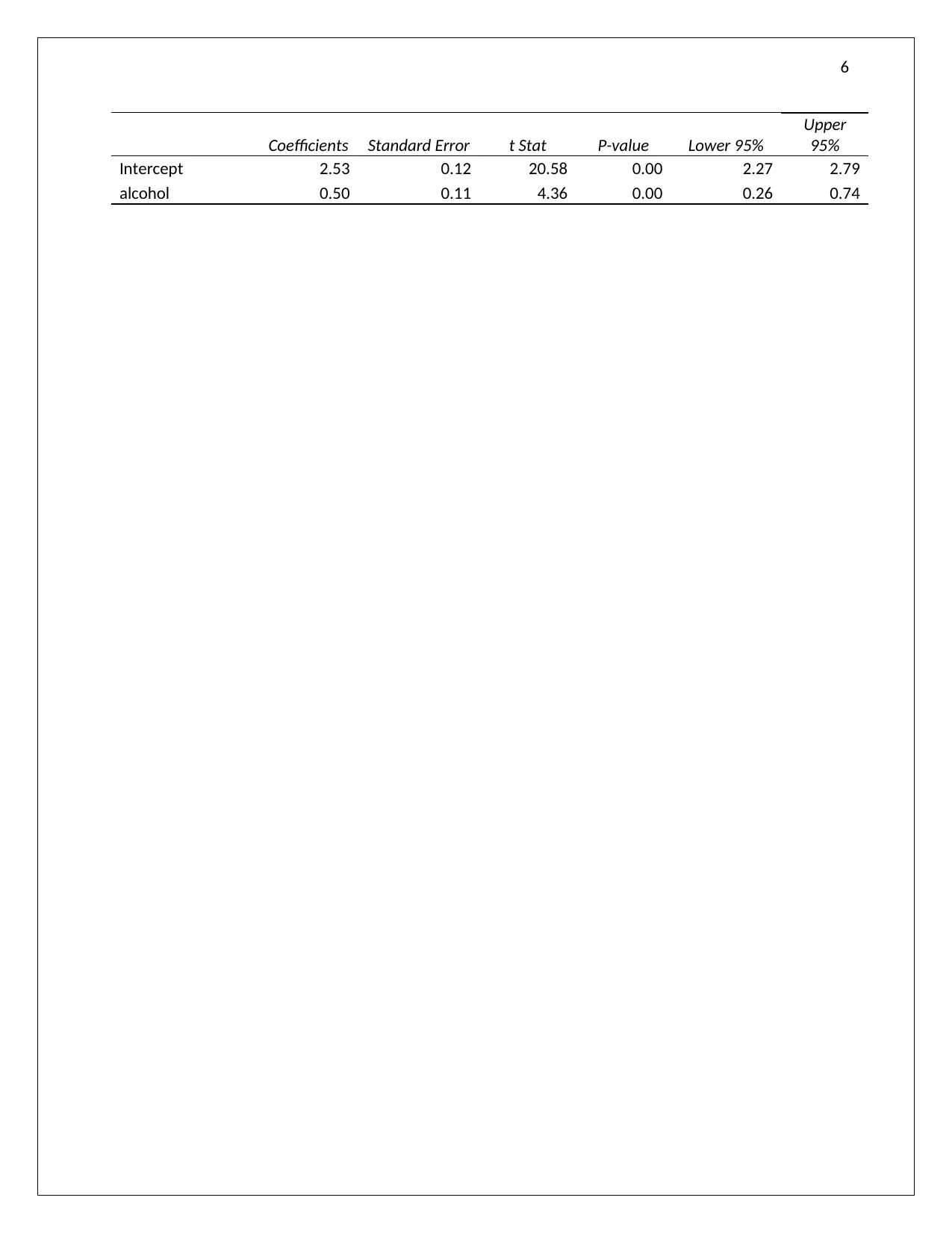
d. ANS: The elasticity of the liver disease deaths due to alcohol consumption was found from re-
calculating the regression model using logarithmic values (detailed model in appendix). The log-
log regression model was evaluated as
ln ( liver ) =2 . 53+0 .5 ln ( alcohol )
. Hence, the elasticity of liver
disease deaths due to alcohol consumption was 0.5. The elasticity of 0.5 signified that, for 1%
change in alcohol consumption, chance of death increased by 50% due to liver disease (Chatterjee
& Hadi, 2015).
Paraphrase This Document
Need a fresh take? Get an instant paraphrase of this document with our AI Paraphraser
5
Reference
Chatterjee, S., & Hadi, A. S. (2015). Regression analysis by example. John Wiley & Sons.
Wooldridge, J. M. (2015). Introductory econometrics: A modern approach. Nelson Education.
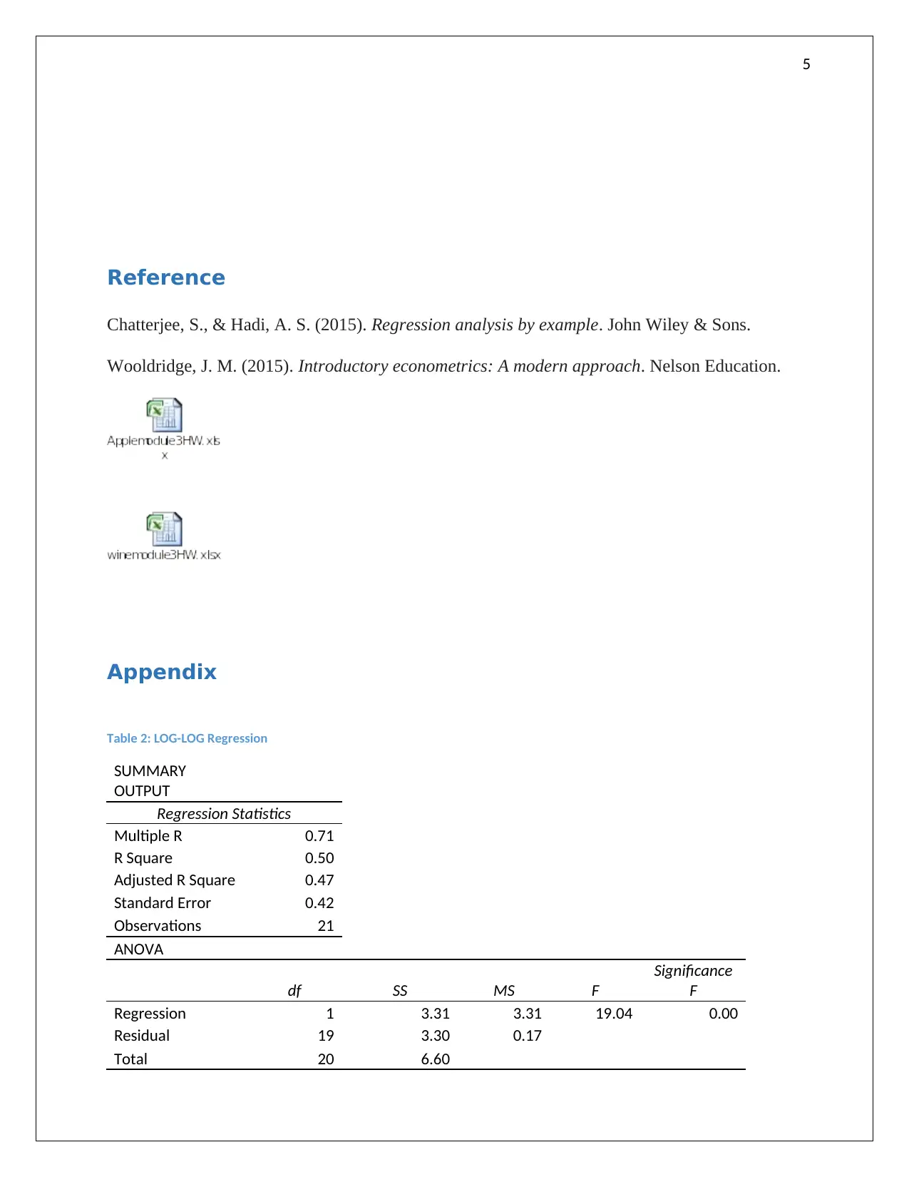
Appendix
Table 2: LOG-LOG Regression
SUMMARY
OUTPUT
Regression Statistics
Multiple R 0.71
R Square 0.50
Adjusted R Square 0.47
Standard Error 0.42
Observations 21
ANOVA
df SS MS F
Significance
F
Regression 1 3.31 3.31 19.04 0.00
Residual 19 3.30 0.17
Total 20 6.60
Reference
Chatterjee, S., & Hadi, A. S. (2015). Regression analysis by example. John Wiley & Sons.
Wooldridge, J. M. (2015). Introductory econometrics: A modern approach. Nelson Education.
Appendix
Table 2: LOG-LOG Regression
SUMMARY
OUTPUT
Regression Statistics
Multiple R 0.71
R Square 0.50
Adjusted R Square 0.47
Standard Error 0.42
Observations 21
ANOVA
df SS MS F
Significance
F
Regression 1 3.31 3.31 19.04 0.00
Residual 19 3.30 0.17
Total 20 6.60
6
Coefficients Standard Error t Stat P-value Lower 95%
Upper
95%
Intercept 2.53 0.12 20.58 0.00 2.27 2.79
alcohol 0.50 0.11 4.36 0.00 0.26 0.74
Coefficients Standard Error t Stat P-value Lower 95%
Upper
95%
Intercept 2.53 0.12 20.58 0.00 2.27 2.79
alcohol 0.50 0.11 4.36 0.00 0.26 0.74
⊘ This is a preview!⊘
Do you want full access?
Subscribe today to unlock all pages.
Trusted by 1+ million students worldwide
1 out of 6
Your All-in-One AI-Powered Toolkit for Academic Success.
+13062052269
info@desklib.com
Available 24*7 on WhatsApp / Email
![[object Object]](/_next/static/media/star-bottom.7253800d.svg)
Unlock your academic potential
© 2024 | Zucol Services PVT LTD | All rights reserved.