Wage and Education Relationship Analysis

This assignment presents a quantitative analysis exploring the relationship between wages and years of education. The study utilizes regression analysis to estimate the impact of education on wage rates, revealing a positive association. However, the model exhibits limitations due to its simplicity, considering only education as an independent variable and having a small sample size. Despite these constraints, the findings support previous research demonstrating the link between education and higher earnings. The assignment concludes with policy recommendations emphasizing the importance of promoting education for economic growth.

Running Head: ECONOMICS AND QUANTITATIVE ANALYSIS
Economics and Quantitative Analysis
Name of the Student
Name of the University
Author note

1ECONOMICS AND QUANTITATIVE ANALYSIS
Table of Contents
1. Purpose...................................................................................................................................2
2. Background............................................................................................................................2
3. Method...................................................................................................................................3
4. Results....................................................................................................................................3
4.1 Descriptive Statistics........................................................................................................3
4.2 Scatter diagram.................................................................................................................4
4.3 Regression estimate..........................................................................................................5
4.4 Goodness of fit.................................................................................................................6
4.5 Predicted wage.................................................................................................................6
5. Discussion..............................................................................................................................7
6. Recommendation....................................................................................................................8
7. References..............................................................................................................................9

2ECONOMICS AND QUANTITATIVE ANALYSIS
1. Purpose
The report aims to find out how education is related with wage level. There can be
both way relation between education and wage. High education generally means a high wage.
Similarly, higher wage by raising income make education affordable for worker. The report
evaluates the impact of education on wage level using linear regression relationship. Based
on the relationship between education and wage suitable policy recommendation can be
developed.
2. Background
Different strategies are taken to stimulate capacity of the individual to succeed in
labor market. Making investment to enrich human capital is one of the important tool to attain
this objective. Several studies have conducted to validate the relationship between wage and
education. Education is the only tool that can enhance a complete development of mind and
shape physical and moral characters. Education helps to gather knowledge, which in turn
contributes to develop technical skills and enhances productivity. The intellectual skills
attained through education is reflected in the work in which the workers engage (Barros and
Ramos 2015). The formal education forms the basis of any technical or skill education.
Education combines with individual ability makes an individual eligible for a standard job.
Wage is the payment made against the work effort given by the workers. Wage
usually depends on the productivity of workers. Workers will high skills are highly
productive. By exploring their productive capacity, they yield a high return to the employers
in the form of high output. Wage in general is determined from the equilibrium in labor
market where labor supply and labor demand balances. Employers always want to have a
skilled workforce and for this, they often offer wage above equilibrium called the efficiency

3ECONOMICS AND QUANTITATIVE ANALYSIS
wage (Andini 2017). Therefore, in general a direct positive relation exists between education
and income.
Based on the assertion that education positively influence wage, economists have
made research to evaluate the proposed relation (Smith and Fernandez 2017). Evaluation of
wage-education relation attracts attention of the researchers to make any policy suggestion in
this aspect.
3. Method
The variables taken for analysis are wage and education. A sample of size 100 are
taken to estimate the relationship between wage and education. A continuous data is collected
on wage while the data on education is discrete in nature. The objective of this paper is find
the association between education and wage. Before estimating relationship between the two
variables, a descriptive analysis is made. The descriptive analysis shows mean, standard
deviation, maximum, minimum and other relevant variables. Then a scatter diagram is
constructed to evaluate relationship between the two quantitative variables at a glance. The
relationship depicted with scatter plots needs statistical confirmation. A regression model is
developed using wage as dependent variable and education as independent variable (Fox
2015). The regression output gives an estimated relationship between the variables in terms
of statistical significance. The goodness of fit of the model is to be determined from the R
square measure. Finally, the estimated model is used to predict wage for the given level of
education.
4. Results
4.1 Descriptive Statistics
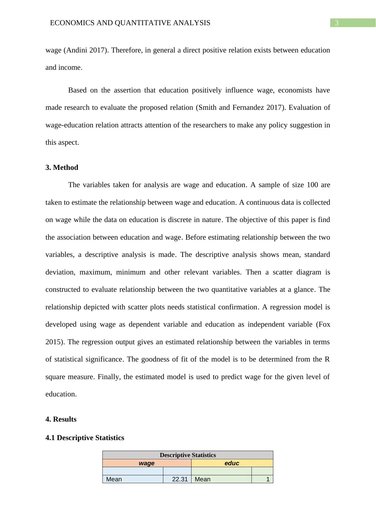
Descriptive Statistics
wage educ
Mean 22.31 Mean 1

4ECONOMICS AND QUANTITATIVE ANALYSIS
3.76
Standard Error 1.40 Standard Error 0.27
Median 19.39 Median
1
3.00
Mode 38.45 Mode
1
2.00
Standard
Deviation 14.02
Standard
Deviation 2.73
Sample Variance 196.60 Sample Variance 7.44
Kurtosis 2.61 Kurtosis 1.32
Skewness 1.49 Skewness 0.44
Range 72.06 Range 15
Minimum 4.33 Minimum 6
Maximum 76.39 Maximum 21
Sum
223
0.81 Sum 1376
Count 100 Count 100
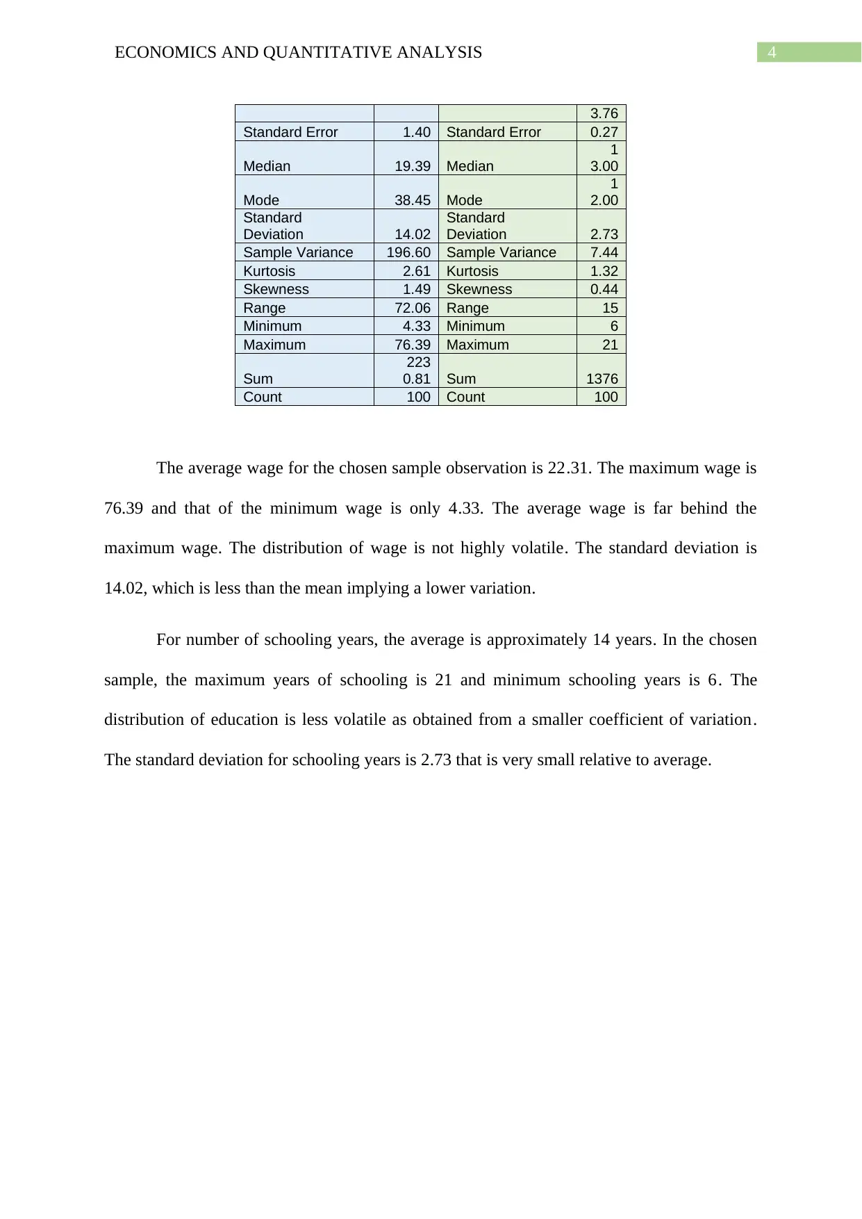
The average wage for the chosen sample observation is 22.31. The maximum wage is
76.39 and that of the minimum wage is only 4.33. The average wage is far behind the
maximum wage. The distribution of wage is not highly volatile. The standard deviation is
14.02, which is less than the mean implying a lower variation.
For number of schooling years, the average is approximately 14 years. In the chosen
sample, the maximum years of schooling is 21 and minimum schooling years is 6. The
distribution of education is less volatile as obtained from a smaller coefficient of variation.
The standard deviation for schooling years is 2.73 that is very small relative to average.

5ECONOMICS AND QUANTITATIVE ANALYSIS
4.2 Scatter diagram
4 6 8 10 12 14 16 18 20 22
0
10
20
30
40
50
60
70
80
90
f(x) = 2.1237563837879 x − 6.91478784092146
R² = 0.170611590067958
Scatter Plot
Education
Wage
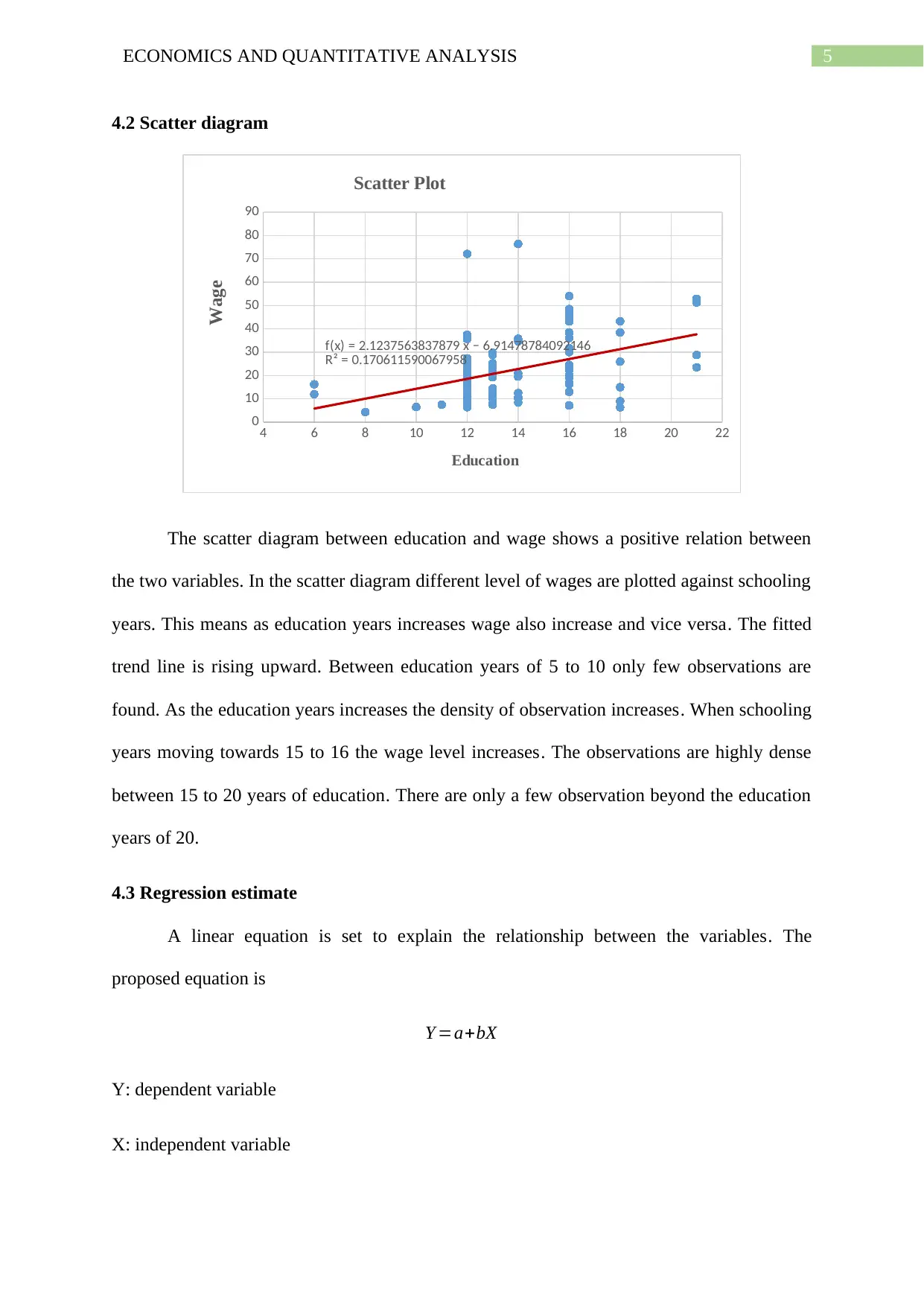
The scatter diagram between education and wage shows a positive relation between
the two variables. In the scatter diagram different level of wages are plotted against schooling
years. This means as education years increases wage also increase and vice versa. The fitted
trend line is rising upward. Between education years of 5 to 10 only few observations are
found. As the education years increases the density of observation increases. When schooling
years moving towards 15 to 16 the wage level increases. The observations are highly dense
between 15 to 20 years of education. There are only a few observation beyond the education
years of 20.
4.3 Regression estimate
A linear equation is set to explain the relationship between the variables. The
proposed equation is
Y =a+bX
Y: dependent variable
X: independent variable

6ECONOMICS AND QUANTITATIVE ANALYSIS
a: intercept
b: slope co-efficient
Regression Statistics
Multiple R 0.41
R Square 0.17
Adjusted R Square 0.16
Standard Error 12.83
Observations 100
ANOVA
df SS MS F Significance F
Regression 1 3320.69 3320.69 20.16 0.00
Residual 98 16142.78 164.72
Total 99 19463.47
Coefficient
s
Standard
Error t Stat
P-
value Lower 95%
Upper
95%
Intercept -6.9148 6.6339 -1.0423 0.2998 -20.0795 6.2500
educ 2.1238 0.4730 4.4899 0.0000 1.1851 3.0624
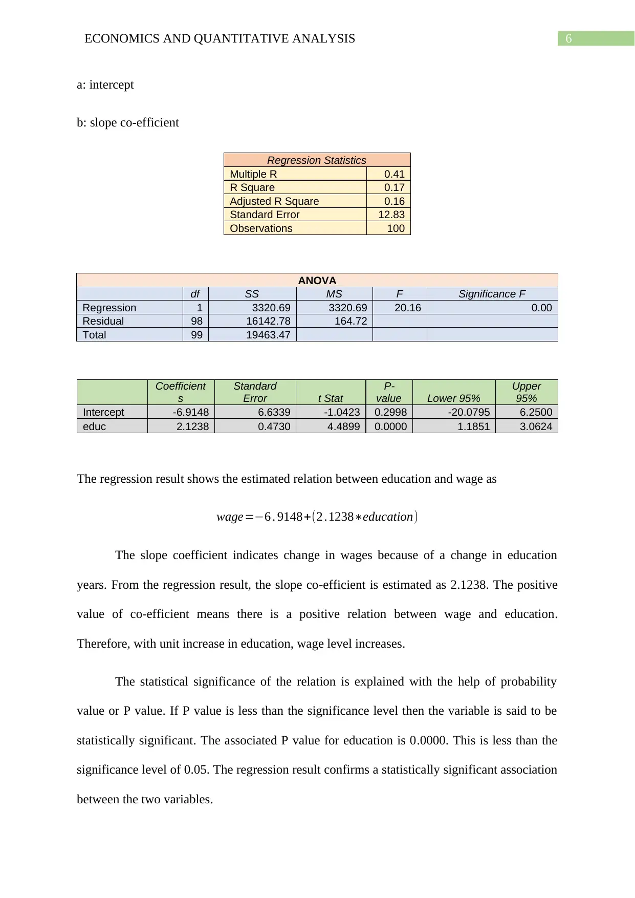
The regression result shows the estimated relation between education and wage as
wage=−6 . 9148+(2 .1238∗education)
The slope coefficient indicates change in wages because of a change in education
years. From the regression result, the slope co-efficient is estimated as 2.1238. The positive
value of co-efficient means there is a positive relation between wage and education.
Therefore, with unit increase in education, wage level increases.
The statistical significance of the relation is explained with the help of probability
value or P value. If P value is less than the significance level then the variable is said to be
statistically significant. The associated P value for education is 0.0000. This is less than the
significance level of 0.05. The regression result confirms a statistically significant association
between the two variables.

7ECONOMICS AND QUANTITATIVE ANALYSIS
4.4 Goodness of fit
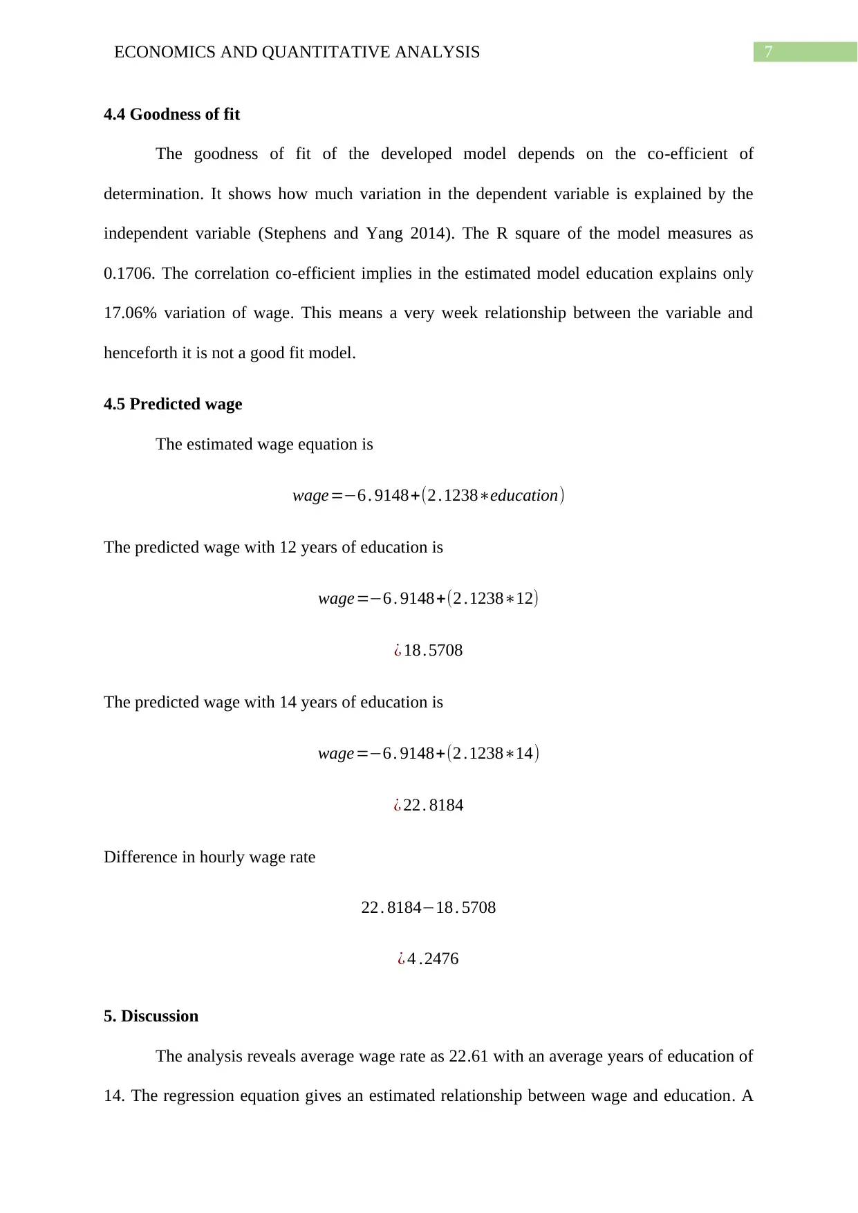
The goodness of fit of the developed model depends on the co-efficient of
determination. It shows how much variation in the dependent variable is explained by the
independent variable (Stephens and Yang 2014). The R square of the model measures as
0.1706. The correlation co-efficient implies in the estimated model education explains only
17.06% variation of wage. This means a very week relationship between the variable and
henceforth it is not a good fit model.
4.5 Predicted wage
The estimated wage equation is
wage=−6 . 9148+(2 .1238∗education)
The predicted wage with 12 years of education is
wage=−6 . 9148+(2 .1238∗12)
¿ 18 .5708
The predicted wage with 14 years of education is
wage=−6 . 9148+(2 .1238∗14)
¿ 22 . 8184
Difference in hourly wage rate
22 . 8184−18 . 5708
¿ 4 .2476
5. Discussion
The analysis reveals average wage rate as 22.61 with an average years of education of
14. The regression equation gives an estimated relationship between wage and education. A

8ECONOMICS AND QUANTITATIVE ANALYSIS
significantly positive relation exists between the two variables. However, the model is not a
good fit model as reflected from a relatively small value of R square.
The key strength of the quantitative research analysis is that results obtained from the
samples can be generalized for the entire population given the sample is chosen precisely and
is well designed. The results are relatively easy to interpret and the selected data can be
consistent if obtained from reliable source.
The first weakness of the research method is the small size of sample. Only 100
observations are chosen. In modeling wage, only education is taken as independent variable.
However, several other variables like gender, experience can influence wage as well but are
not included in the model.
The findings of the paper shows support to research results of previous studies. Many
scholarly studies have found a positive association between wage and education and that of
the productivity gains (Popescu and Militaru 2017). The result of the present paper and other
related studies provides strong policy support towards promoting education to enhance
average income.
6. Recommendation
The paper finds a positive association between wage and education. Therefore,
government should undertake policies to promote education in countries. Especially,
government in developing nations should mandate school enrollment. Implementation of
rules is not sufficient. Government should arrange campaigns to aware people regarding the
importance of education in influencing wage. Apart from formal education, technical
education should be provided to develop skill.

9ECONOMICS AND QUANTITATIVE ANALYSIS

10ECONOMICS AND QUANTITATIVE ANALYSIS
7. References
Andini, C., 2017. Tertiary Education for All and Wage Inequality: Policy Insights from
Quantile Regression (No. 132). Institute for the Study of Labor (IZA).
Barros, R.P.D. and Ramos, L., 2015. A note on the temporal evolution of the relationship
between wages and education among Brazilian prime-age males: 1976-1989.
Fox, J., 2015. Applied regression analysis and generalized linear models. Sage Publications.
Popescu, M.E. and Militaru, E., 2017. Education and Wage Inequalities under a
Counterfactual Scenario of Minimum Wage. Acta Universitatis Danubius.
Œconomica, 13(6).
Smith, W.C. and Fernandez, F., 2017. Education, Skills, and Wage Gaps in Canada and the
United States. International Migration, 55(3), pp.57-73.
Stephens, M. and Yang, D.Y., 2014. Compulsory education and the benefits of
schooling. The American Economic Review, 104(6), pp.1777-1792.